
Simulations of Blood Drop Spreading and Impact for Bloodstain Pattern Analysis
2014-04-17 11:06:05ChuWangandLucyZhang
Chu Wang and Lucy T.Zhang
1 Introduction
The bloodstain pattern analysis(BPA),which is a part of the forensic science,can be crucial in solving a crime scene[Karger,Rand,Fracasso,and Pfeiffer(2008)].It provides more comprehensive evidence for criminologists and scientists by an-alyzing blood generation,motion and spatter patterns.In the most recent review article on fluid dynamics and bloodstain pattern analysis,Attinger et al.[Attinger,Moore,Donaldson,Jafari,and Stone(2013)]addressed the essential role fluid dynamics plays in forensic science.In both communities,BPA and fluid dynamics,the blood drop dynamics as it interacts with surrounding environments,air and/or other liquids or solids,has always been one of the key components of the analysis.The underlying physics of these multi-phase interactions involve blood drop trajectories in air(multi- fluid flows)and the spatter patterns(blood spatter analysis)as blood drops impact on solid surfaces( fluid-solid interactions).Therefore, fluid dynamic analysis,focusing on multiphase flows such as the studies of drop impact and spreading,can be used to perform BPA considering the similarities drawn between the two[Attinger,Moore,Donaldson,Jafari,and Stone(2013)].
Among the many possible dominant factors such as drop generation,trajectories,impact,staining patterns on different types of surfaces in analyzing blood drops and blood stains,here we will only focus our effort on two of them:(1)drop spreading,and(2)drop impact.Numerical model and simulations of blood drop spreading and impact can offer scientists a visual and dynamic prediction on the exact sequence of events.However,the complicated behaviors of blood drops require the numerical models to be capable of accurately capturing and predicting the intricate interplay among the interfacial forces,which include:(a)the three-phase(air-liquid-solid)dynamic contact line,(b)solving the Navier-Stokes equations with properly modeled surface tension force,and(c)coping with geometry topology changes of the blood drops during the process,such as blood spattering due to impact.
In the forefront of modelingdrop spreading,which involves the overall surface energy balance among air-liquid,liquid-surface,and air-surface,several numerical algorithms have been proposed and widely used,such as the front tracking method[Tryggvason,Bunner,Esmaeeli,Juric,Al-Rawahi,Tauber,Han,Nas,and Jan(2001);Unverdi and Tryggvason(1992);Witteveen,Koren,and Bakker(2007);Muradoglu and Tryggvason(2008)],volume of fluid method(VOF)[Hirt and Nichols(1981);Cervone,Manservisi,and Scardovelli(2010)]and the level-set method[Xu,Li,Lowengrub,and Zhao(2006);Herrmann(2008)].The classic usage of these methods is only to model air-liquid multiphase flows,which sets the limitations of their applicability.Drop spreading and impact are dynamic processes that also involve the interactions with solid surfaces.Therefore, fluid(air/gas or liquid)interacting with solid surfaces must also be accounted for in these simulations.This then introduces the concept of“contact line”.
Direct simulations of fluid interacting with solid boundaries encounters a mathematical dilemma in capturing the moving contact line along a no-slip boundary:the fluid velocity is finite at the free-surface but zero on the solid surface[Dupon-t and Legendre(2010)].Therefore a stress singularity is formed.The divergent stress comes from the fact that the continuum assumption of the fluid is no longer valid within the molecular length scale near the three phase contact region.The molecular interactions between the fluid and the solid within the molecular length scale are required in the model.Besides direct simulations,there are various numerical models to deal with the contact line problem.To apply a non-slip boundary condition on a solid surface,one of the models suggests[Di and Wang(2009)]to assume there is a thin liquid film as a precursor model.The singular stress is naturally removed if the inclusion of a microscopic precursor film is placed in front of the apparent contact line.However,the assumption of the existence of the thin liquid film is under debate because if it does exist,it is generally not fast enough to stay ahead of the contact line[Chen,Mertz,and Kulenovic(2009)].Other studies have been made to address this problem by relaxing the no-slip boundary condition with a slip boundary model to resolve the singular stress when solving the Navier-Stokes equations.Due to the lack of description of the microscopic interactions between the fluid and solid in the subgrid scale,the contact angle typically needs to be specified from some empirical models to treat the contact line.Many multiphase simulating techniques such as front tracking[Muradoglu and Tasoglu(2010)],level-set[Spelt(2005);Chen,Mertz,and Kulenovic(2009)],VOF[Sikalo,Wihelm,and Roisman(2005);Afkhami,Zaleski,and Bussmann(2009)]have adopted this approach to simulate contact line problems successfully.The contact angle is either imposed to the explicit interfacial markers at the contact line(front tracking method)or specified as a boundary condition(level-set and VOF).Despite the limitation of the results been dependent on the slip-length and thus on the grid spacing,the method is still widely adopted due to its simplicity and easiness to implement into an existing multiphase flow algorithm.
The biggest challenge here,however,is modeling thedrop impact,where a drop impacts on a solid surface and upon impact,the drop spatters into small drops.In other words,the topology,or the geometry of the interface of the drop changes as the drop breaks up.To handle topology changes numerically is not a trivial task because of the connectivities among the points that represent the interface cannot be maintained through time.The re-construction and re-connecting of the drop interface as it goes through dramatic changes can be quite daunting.In our recent development,we proposed a connectivity-free front tracking(CFFT)method[Wang,Wang,and Zhang(2013)].The main goal of this development was to handle topology changes of the interfacewithoutthe constraint of the connectivities of the interfacial points,therefore the name “connectivity-free”.It combines the merits of the front tracking and front capturing approaches such that explicit interfacial points were used for interface representation to achieve better volume conservation,and constructing a smooth and accurate indicator field based on the actual location and geometry of the interface for fluid properties(curvature and surface tension)calculations.
Naturally,to successfully model drop spreading and impact involves two main features to be included in an algorithm:(1)a multiphase model without connectivity to handle drop breaking-up or spattering,and(2)a fluid-solid contact line model that accurately captures the contact line dynamics.The objective of this paper is to couple a dynamic contact line model into the CFFT algorithm so that drop spreading and impact can be studied and analyzed.To our knowledge,this is a first attempt in coupling a contact line model into a connectivity-free multiphase method.To demonstrate the capabilities of this coupled algorithm,several numerical experiments are examined in 2-D.Three-dimensional problems are not particularly difficult in either contact line model or CFFT algorithm individually,in fact they have been examined independently for 3-D problems[Shi,Bao,and Wang(2013);Wang,Wang,and Zhang(2013)]even though contact line model was mostly modeled with axis-symmetric and 2-D[Dupont and Legendre(2010)].However,the combination of the two involves quite complex 3-D surface reconstruction algorithm,which requires significantly more effort.Here,our main focus is to first develop the numerical framework,the 3-D implementation is to be completed in the near future.
Under the framework of the CFFT method,the points regeneration scheme can cope with the interface topology change automatically,and construct the initial contact line by connecting points to the solid surface when the interface is close enough.The dynamic contact line model then reconstructs the contact by adjusting the explicitly represented interface.Coupling the contact line model to CFFT has many advantages:1)No connectivities required for the interfacial points which is hard to maintain when interface undergoes topology change;2)The break-up and coalescence,and the initial contact line formation can be automatically treated with a points-regeneration scheme;3)Easy implementation of the dynamic contact line model with the interface represented by explicit points;4)Avoid solving the advection equation in the VOF and level-set method which would require special treatment to deal with issues related to stability and volume conservation.
The outline of this paper is as follows.In Section 2,the mathematical model is presented.We first review the governing equation of the connectivity-free front tracking method and then discuss the treatment of the moving contact line with proper empirical correlations between the contact angle and the capillary number.In Section 3,three numerical examples are studied to validate the algorithm.Finally,the conclusions are drawn in Section 4.
2 Numerical Algorithm
2.1 The connectivity-free front tracking method
A ‘one fluid’approach is used to describe the multi- fluid flow regime[Hua,Stene,and Lin(2008)],which uses only a single set of Navier-Stokes equations with fluid properties varying across the interface without the need to treat the pressure jump condition.Both fluids(air and liquid)are considered as isothermal,incompressible flow.The surface tension force is added to the momentum equation as a singular force term.The overall governing equations are expressed as follows:
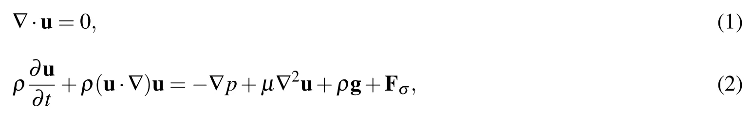
where u is the velocity,pis the pressure,ρ and μ are the fluid density and viscosity,respectively,g is the gravity,and Fσis the surface tension force.
The fluid properties(density ρ and viscosity μ)are calculated using an indicator defined asI=1 for liquid andI=0 for air.A linear interpolation is used to perform the calculation:
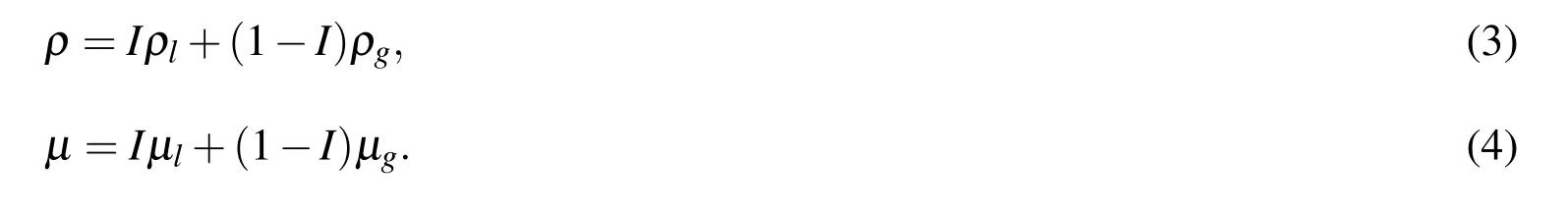
The subscriptslandgdenote the liquid and air,respectively.
In the front tracking method[Unverdi and Tryggvason(1992)],the indicator field near the interface is obtained by solving the Poisson’s equation:
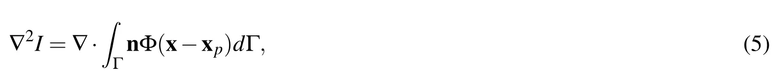
where Γ is the interface,Φ is an appropriate interpolation function and n is the unit normal,which requires to be obtainedaprioriutilizing the connectivity of the interfacial points.The connectivity of the interfacial points is sometimes difficult to maintain when the interface undergoes frequent topology changes,especially when the air-liquid starts to contact with a solid surface generating a three-phase contact,which requires the interface connectivity to be reconstructed constantly.It is even more complicated for 3-D cases.
The CFFT method adopts an alternative way to cope with the necessity of connectivity[Wang,Wang,and Zhang(2013)].It still uses the explicit interfacial points to describe and update the interface where a good volume conservation can be achieved in a divergence-free incompressible flow field[Tryggvason,Bunner,Esmaeeli,Juric,Al-Rawahi,Tauber,Han,Nas,and Jan(2001)].However,by combining the basic concept of the front capturing methods such as level-set method and the VOF method,the indicator field is obtained first using the un-connected interfacial points through a special treatment,the unit normal and curvature are then calculated from the indicator field.
The procedure of obtaining the indicator without interfacial points connectivity is as follows:obtain an approximate indicator field first and then correct this indicator field based on the current position of the interfacial points.In order to achieve this,we first define a set of ghost points()that are placed at the center of each fluid element(see Fig.1).Noting that this is different from the original CFFT where a ghost fluid mesh instead of points is constructed.Without the mesh,it adds flexibility when constructing the indicator.One can simply use more points within each fluid element to achieve better resolution.If the initial position of the interface is known,the approximate indicator for the ghost points at the beginning of the simulation is also known.
In the front capturing method,the indicator or signed distance function is advected by solving an advection equation(6)implicitly at the current time step:

Solely using advection equation to update indicator function may cause issues in stability and volume conservation.Here we use it to acquire the approximate indicator fieldIaat the current time stepnexplicitly by evaluating the indicator for each ghost point based on the previous time step indicator fieldIn?1and interface velocityun?1:

Since the ghost points are defined arbitrarily and their indicator values are explicitly solved,it provides the possibility to increase or decrease the ghost point resolution when needed.
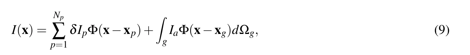
Once the approximate indicator field,Ia,is obtained for the ghost points,we can interpolate the indicator field from the ghost points,xgto any point x,such as the fluid nodes and the interfacial points,through a proper delta function,Φ:

Once the indicator values on the interfacial points are found,we then correct it so that the interface would have a constant indicator(level).In order to achieve this,a correction term δIp(xp)for each interfacial point,p,is added to Eq.(8)when performing the interpolation:
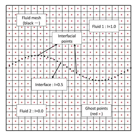
Figure 1:Schematics of computational domain set up.
where the subscriptpdenotes the interfacial points,Npis the number of interfacial points.The correction term needs to be solved for every interfacial point,p.If the indicator of all the interfacial points is set to be 0.5,i.e.I(xp)=0.5,then
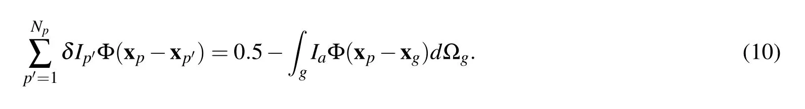
Here the subscriptp0is used to differentiate frompin the summation.Solving Eq.(10)yields the correction value δIpfor each interfacial point.Once the correction of the indicator function is solved,the final indicator field for the fixed fluid mesh can be obtained using Eq.(9).
The surface tension force is calculated using a continuum surface tension force(CSF)approach[Brackbill,Kothe,and Zemach(1992)],which can convert the sin-gular point/surface force into volume force that spans the vicinity of the interface:

where[I]is the jump of the indicator function and<ρ>is the average density at the interface.
To make sure the interpolation is performed accurately for near solid surface region where the influence domain is incomplete,the reproducing kernel particle method(RKPM)interpolation scheme is chosen[Liu,Jun,and Zhang(1995);Liu,Jun,Li,Adee,and Belytschko(1995)].The use of a higher order interpolation function and the satisfaction of the reproducing condition are essential in accurately calculating the normal and curvature of the interface,hence in forming a correct contact line.The details of the RKPM implementation can be found in[Wang,Wang,and Zhang(2013)].
Once the indicator field is constructed and the surface tension force is calculated,the Navier-Stokes equations are then solved to obtain the velocity and pressure fields.The interface is updated using the velocity at each interfacial point u(xp),which is interpolated from the fluid mesh:

wherenis the current time step,n+1 is the next time step,and?tis the time step size.
During the evolution of the interface,the interfacial points often need to be regenerated for the following purposes:1)to maintain sufficient points within each interfacial segment;2)to handle topology changes when both the breaking-up and coalescence occur by adding or deleting points near the contact;3)to form the initial contact line by connecting the nearby interfacial points to the solid surface.The regeneration of the interface is achieved by carefully selecting some points inside the fluid elements near the interface as the candidate points and projecting them onto the interface.The point projection scheme is described as follows.We first consider a candidate point at the position x with indicator valueI(x),then project the point onto the interface along the normal direction of the indicator.We allow x to move δx so that the indicator of the candidate point achieves 0.5.
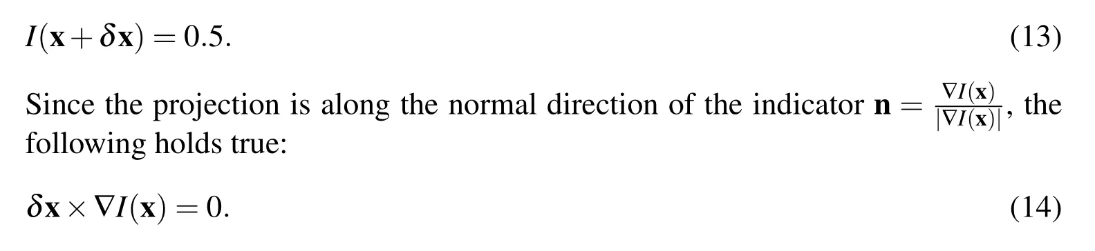
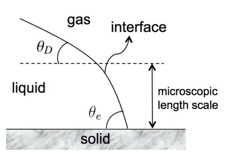
Figure 2:Contact line dynamics.
Based on Eqs.(13)and(14),δx is solved and the candidate point is projected to a new position x0=x+δx.This scheme is performed several times until|I(x0)?0.5|< ε,where ε is a set tolerance,then a new interfacial point is regenerated.The interface topology changes and the formation of initial contact line are treated by selecting candidate points from alternate side of the interface to ensure the breaking-up and coalescence of the interface are properly treated.The detailed description on the points-regeneration scheme can be referred to[Wang,Wang,and Zhang(2013)].
2.2 Dynamic contact line model
The dynamics of the contact line in our study can be described as follows.At the microscopic length scale,the contact angle of a moving interface is a constant,which is equal to the equilibrium contact angle θe(see Fig.2).The contact angle is known for a given air-liquid-solid system.Since our numerical simulation does not directly account for the molecular interactions of the three phases at the microscopic length scale,we use the so-called ‘a(chǎn)pparent’dynamic contact angle which defines the macroscopic relation between the contact line and the solid surface.A dynamic contact line model is needed here to relate the dynamic contact angle and the microscopic interactions of the three phases.
To apply no-slip boundary condition on the solid surface would yield a stress singularity at the contact line.To avoid this problem,a Navier-slip boundary condition is imposed so that the fluid is allowed to slide along the solid surface:
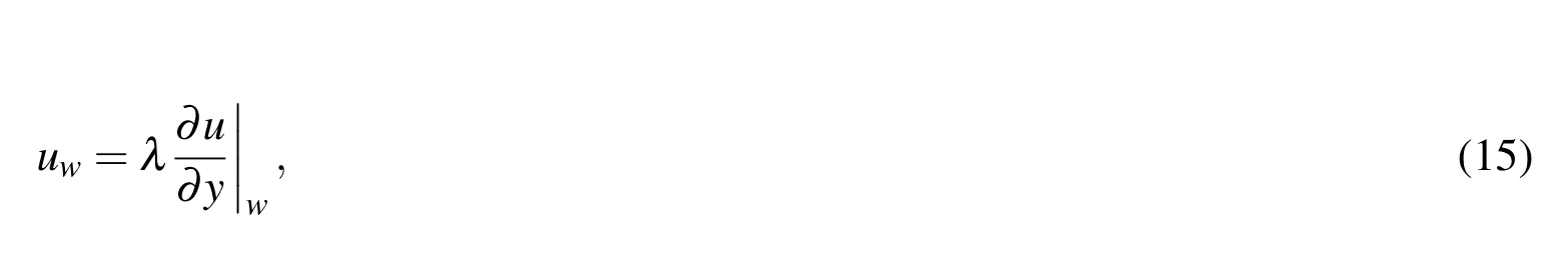
whereuwis the fluid velocity on the solid surface,and λ is a pre-defined sliplength for a given problem.In reality,the true slip-length is in the order of the intermolecular distance,here we choose λ=0.001 for all the numerical examples,which does not allow too much movement of the contact line.
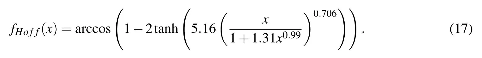
The shape of the contact line is dependent on the contact angle formed with the surface and the intrinsic properties of the liquid.An empirical model is demanded here to reconstruct the contact line by correlating the dynamic contact angle and the capillary number.The model we use is first presented by Kistler[Kistler(1993)]and is widely used in other studies[Muradoglu and Tasoglu(2010);Mukherjee and Abraham(2007);Sikalo,Wihelm,and Roisman(2005);Roisman,Opfer,Tropea,Raessi,Mostaghimi,and Chandra(2008)].It is proven to be suitable in dealing with contact line movement:

Cacl= μUcl/σ(Uclis the capillary number of the contact line;Uclis the velocity of the contact line. θeis the equilibrium contact angle.fHoffis the Hoffman’s function which is defined as:
Due to hysteresis,the contact line can only advance when the contact angle is beyond the advancing contact angle θA,or recede when the contact angle is below the receding contact angle θR.If θAand θRare prescribed for a particular system,the dynamic contact angle θDcan still be computed using Eq.(16)by substituting θewith θA(when advancing)or θR(when receding).
Under the framework of the connectivity-free front tracking method,the interface is explicitly presented by interfacial points.Once the interface gets close enough to the solid surface,the points-regeneration scheme starts to connect the interfacial points to the surface to form an initial contact line.Therefore,the remaining task is to use the empirical model to reconstruct the initial contact line and predict the correct movement.
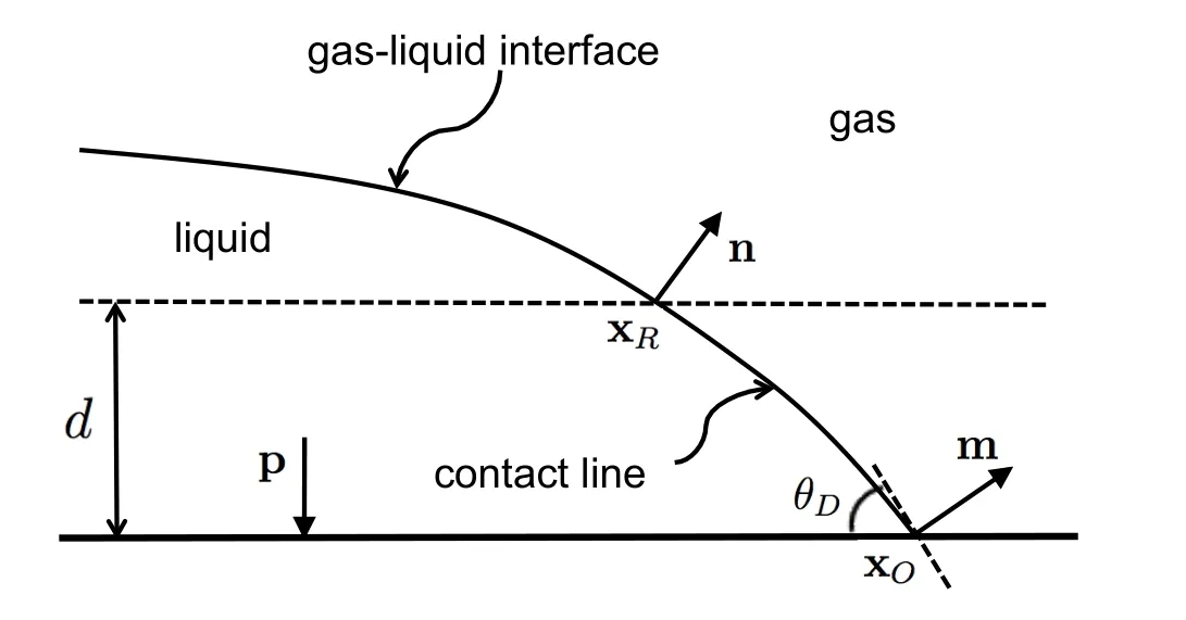
Figure 3:Schematics of contact line construction.
The schematics of the contact line construction is shown in Fig.3.At each time step,if the interfacial points are found to be connected to the solid,the contact line needs to be reconstructed so that the unit normals of the interfacial points connecting to the solid surface obey the predicted dynamic contact angle using Eq.(16).To determine the dynamic contact angle θD,the contact line velocityUclmust be specified.To use the velocity of the three-phase contact point xOas the contact line velocity,an iterative procedure would be required to determine the location and the velocity of the three-phase contact point since each of them is affected by the other.The iteration would not reach convergence when the contact line velocity approaches zero[Muradoglu and Tasoglu(2010)].Here we let the tangential(to the surface)component of a reference point velocity vRto be the velocity of the contact lineUcl.The reference point xRis located at a distancedfrom the solid surface.The distance can be specified asd=ε?x,where?xis the grid spacing,ε is a scaling factor specified as 0.9 arbitrarily.This reference point is explicitly generated during the regeneration scheme.The unit normal nRand velocity vRfor this particular point can also be calculated.To determine whether the contact line is advancing or receding,simply evaluate the sign of vR·nR.The unit normal for each interfacial point is defined to be along the outward normal direction.Therefore,if vR·nR>0,then the contact line is advancing;if vR·nR<0,then the contact line is receding.
Once the contact line velocity is determined,the dynamic contact angle,hence the unit normal for the point connected to the solid surface,can be calculated from Eq.(16).The contact line is reconstructed using an arc from a perfect circle.The advantage to use an arc to fit is that the outward unit normal can transit smoothly from the reference point xRto the end point of the contact line xO.For a 2-D construction,assuming the coordinates(xR,yR)and the unit normal(nx,ny)for the reference point are known.The unit normal of the point connected to the solid(mx,my)is calculated from the dynamic contact angle.The outward normal for the solid surface is denoted as(px,py).The goal is to find the coordinates of the last point of the contact line(xO,yO).Because the reference point and the last point are along the same circle,assuming the center of the circle is located at(xC,yC),then the following equations must be satisfied:
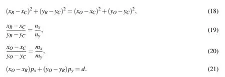
To rule out any unrealistic solutions,the following condition must be satisfied:

Based on the conditions(18)to(22),the coordinates at the point of contact,or the last point of the contact line are calculated.More interfacial points can be added between the reference point and three-phase contact point following the arc,providing a smooth reconstructed contact line.
The method can be easily extended to the 3-D case.Whenever a reference point is selected and its unit normal is obtained,the contact line is constructed in the plane formed by the unit normal of the reference point(n)and the normal of the solid surface(p),similar to the 2-D contact construction.The actual locations of the newly constructed points can be obtained by transforming the coordinates from the 2-D plane to the 3-D space.
Once the contact line construction is completed,a smooth indicator field is then obtained following the CFFT method.With accurate evaluations of the interface(contact line)normal by adopting the RKPM interpolation,the following condition can be automatically satisfied:
The subscriptwpdenotes the interfacial point that directly connects the surface.nwpis the unit normal calculated from the dynamic contact angle.Condition(23)is used as a boundary condition for the front capturing method when solving the advection equation.Our approach achieves this condition using a different manner,as described in this section.
2.3 Numerical procedure
The overall numerical procedure can be summarized as follows.
1)Perform the points-regeneration scheme to regulate the interfacial points,deal with the topology changes such as breaking-up and coalescence if occur,and connect the interface to the solid surface when interface gets sufficiently close.
2)If a contact line is detected,calculate the contact angle θ.If θR< θ < θA,the contact line movement is under hysteresis,there is no need to reconstruct.If θ > θAor θ < θR,reconstruct the contact line following the procedure mentioned above.3)Construct a smooth indicator field based on the interface using the CFFT method.4)Calculate the fluid properties and the surface tension force using Eqs.(3),(4)and(11).Solve the Navier-Stokes equations to obtain the velocity and pressure fields for the fluid.
5)Finally,update the interface based on the velocity field asThen go back to step 1)for the next time step.
3 Numerical Examples
The examples to be studied here use non-dimensionalized dimensions and material parameters.
3.1 Drop spreads on a horizontal surface
This numerical study is to examine the spreading of a drop on a horizontal solid surface due to gravity.Opposing to the spreading,the surface tension force tries to maintain the sphericity of the drop.The movement of the contact line is constrained by the dynamic contact angle,where the drop eventually reaches an equilibrium shape.With a given static or equilibrium contact angle(θe),the final shape of the drop can be uniquely determined.
A 2-D circular drop is initially placed on a horizontal surface.The schematic is shown in Fig.4.The computational domain is a 6×2 rectangular box,which is discretized using 53,200 uniform quadrilateral elements.The drop with a radius of 0.5 is placed at the bottom center of the box.The density and viscosity ratios of the liquid drop and the ambient air are ρl/ρg=1000 and μl/μg=100,respectively.To analyze the final shape of the drop,we perform the simulations with and without the dynamic contact line model.For the cases with dynamic contact line model,we perform the simulation for 3 different equilibrium contact angles(θe=60?,90?and 120?)with Eotvos numberEo=1.0.The Eotvos number,Eo= ρlg/σ,represents the ratio of gravity and capillary force,where ρlis the density of the drop,R0is the radius of the initial drop,gis the gravity,and σ is the surface tension.
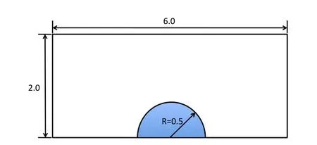
Figure 4:Schematic of a drop spreading on a horizontal plane.
In this example,surface hysteresis is not considered.The final shapes of the drop at equilibrium of these 4 cases (one without the dynamic contact line model and 3 with the dynamic contact line model)are shown in Fig.5.We can observe that when the dynamic contact line model is used,the final shapes of the drop are successfully reproduced for their corresponding equilibrium contact angles.However,when the dynamic contact line model is not used,the drop shape is purely controlled by the gravity and the surface tension force.Without any mechanism to constrain the contact line,the drop shape does not account for any wettability of the surface.In this case,the equilibrium contact angle converges to around 100?.
In order to analyze the effect ofEonumber on the final shapes of the spreading drop,the simulations are performed forEonumber varying from 0.01 to 50,which is achieved by adjusting the ratio of gravity and surface tension.
To further analyze the effect of theEonumber on the final shapes of the spreading drop,the simulations are performed forEonumber varying from 0.01 to 50,which is achieved by adjusting the ratio of gravity and surface tension.WhenEo<<1,the capillary force has a dominant role in the movement of the drop,the shape of the drop cap remains round.According to[Dupont and Legendre(2010)],the maximum height of the dropH0measured from the solid surface is independent ofEo,and can be determined as a function of the equilibrium contact angle as:

WhenEo>>1,the gravity controls the shape of the drop and the maximum heightH∞of the drop is a function of both θeandEonumber:

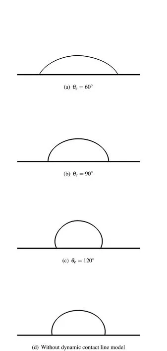
Figure 5:Final shapes of the drop for different equilibrium contact angles and without dynamic contact line model.
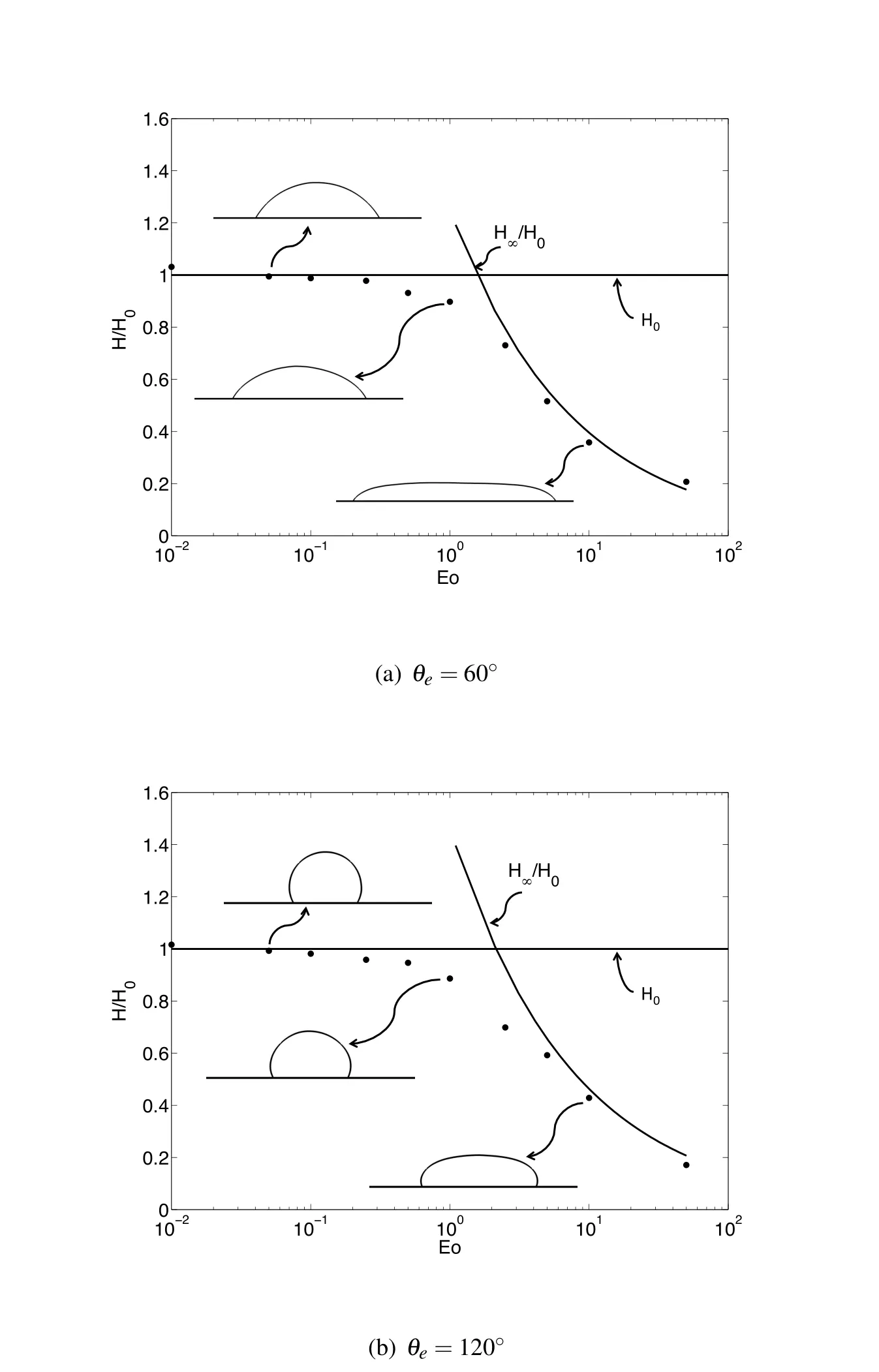
Figure 6:Normalized maximum height vs.Eo.
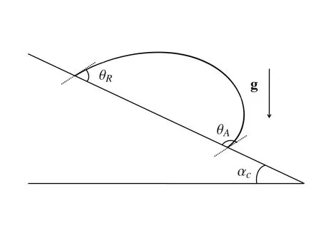
Figure 7:Schematic of a drop moving on an oblique surface.
Here we compare the normalized maximum height of the drop(H/H0)at equilibrium for a large range of Eotvos number(0.01,0.05,0.1,0.25,0.5,1.0,2.5,5.0,10,50)on a hydrophilic(θe=60?)and a hydrophobic(θe=120?)solid surfaces with analytical prediction(Eqs.(24)and(25))in Fig.(6).It can be clearly seen that the computed drop height agrees very well with the asymptotic solutions obtained from Eqs.(24)and(25).The transition of the final shape of the drop from a round cap to a puddled shape asEonumber increased is clearly seen.This simple test shows that the dynamic contact line model that is coupled into the CFFT algorithm can accurately construct the contact line according to a given contact angle.The final shape of the spreading drop can be successfully obtained.
3.2 Drop spreads on an oblique surface
In this example,a drop with hysteresis moving on an oblique surface with variousEonumber is simulated.When the surface inclination angle is at a critical inclination angle αC,the gravity and capillary force balance with each other,which is also called the critical condition(See Fig.7).If the inclination angle of the surface is larger than αC,both the front and the trailing edges of the drop would start to move.The critical inclination angle is also influenced by the given hysteresis angles,and can be calculated as[Dupont and Legendre(2010)]:

whereAis the entire surface area of the 2-D drop. θAand θRare the receding and advancing angles,respectively.The upper caseAandRdenote the predefined advancing and receding contact angles based on hysteresis.We use the lower caseaandrto describe the actual advancing and receding contact angles obtained from the numerical calculation based on the dynamic contact line model.Re-arranging the equation withEonumber we get:

In this set-up,a semi-circular drop is placed on a solid surface.The schematic is the same as previous numerical example.The inclination angle of the solid surface is adjusted by manipulating the direction of the gravity.The density and viscosity ratios of the liquid drop and air are 1000 and 100,respectively.Three sets ofEonumbers 0.5,1 and 2 and two sets of hysteresis angles(θA,θR)=(100?,80?)and(120?,60?)are chosen.The equilibrium contact angle is set to be 90?.For each combination of anEonumber and a set of hysteresis angles,a series of inclination angles with an increment of 5?or 10?near and away from the estimated critical inclination angle are examined using the simulation model.Each simulation is run until the system reaches equilibrium.From the simulations,a critical inclination angle is identified by linear interpolation of inclination angles right before and after the the drop reaches hysteresis.An example is shown in Fig.8 for the combination
Eo=1 and(θA,θR)=(120?,60?).This figure shows the variation of the advancing and receding contact angles for a range of selected inclination angles α from 10?to 90?.When the inclination angle increases,the drop starts to deform in order to maintain a balance between the gravity and the capillary force.The advancing contact angle reaches beyond the hysteresis angle(θA=120?) first and exceeds a little during the rest of the simulation,which agrees with the experimental observation in[ElSherbini and Jacobi(2006)].Similar numerical simulations[Dupont and Legendre(2010)]also confirm this conclusion.The receding contact line starts to move around α =39?,at which point the drop starts to slide due to both the advancing and receding contact lines are moving.The drop shapes when α =20?,40?and 80?are shown in Fig.9.The evolution of the drop and the sliding behavior after the drop reaches the critical condition(α =80?)can be clearly seen.
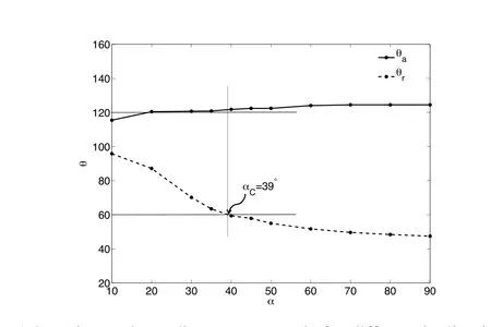
Figure 8:Advancing and receding contact angle for different inclination angles for Eo=1 and(θA,θR)=(120?,60?).

Figure 9:Drop shapes at α =20?,40? and 80? for Eo=1 and(θA,θR)=(120?,60?).
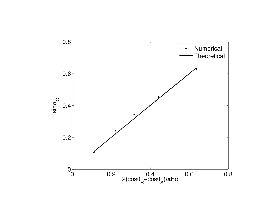
Figure 10:sin αCvs.2(cosθR?cos θA)/πEo.
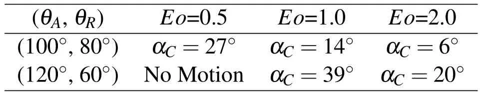
Table 1:Calculated critical angle.
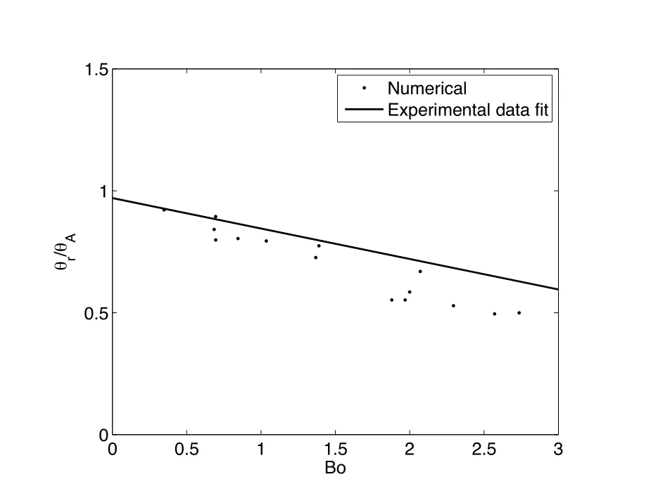
Figure 11:Normalized receding contact angle vs.Bo before the drop reaches critical condition.The experimental data fit is obtained from[ElSherbini and Jacobi(2006)].
The critical angle identified from the simulation for differentEonumber and hysteresis angles are listed in Table(1).We also compare the numerical and theoretical critical angles obtained from Eq.(27),shown in Fig.10.A very good agreement is achieved.For the combination ofEo=0.5 and(θA,θR)=(120?,60?),there is no motion for the drop.That is because during the entire simulation the receding contact angle θrnever reaches the predefined receding contact angle of θR=60?,and the capillary force completely balances with the gravity.Therefore the drop hangs onto the surface.
In a previous work,ElSherbini and Jacobi[ElSherbini and Jacobi(2006)]found a linear relationship between the minimum receding contact angle of a 3-D liquid drop andBonumberbefore the drop reaches the critical condition:

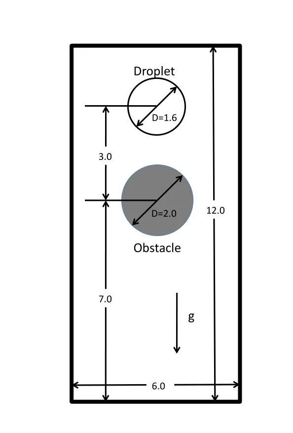
Figure 12:Schematics of a drop impacts on a solid surface.
This relationship is based on the experimental data using various testing surface,liquid,drop size,and inclination angle combinations,which result in different hysteresis angles and liquid properties.To see if our simulation can reproduce this relationship,we plot the non-dimensionalized receding contact angle θr/θAfor variousBonumbers before the drop reaches the critical condition in Fig.11.We may notice that θr/θAdecreases almost linearly whenBoincreases,which is consistent with the linear relationship obtained from the experimental data.However,the experiment is performed for 3-D drops with θrbeen the minimum receding contact angle and the experiment θAbeen restricted to from 49?to 112?.Those factors could be the reasons for the small discrepancy of the simulated results and the linear fit from the experimental data.
3.3 Drop impacts on a solid
To show the robustness of the implementation,we simulate a more complicated case with a drop impacting onto a round solid obstacle.The geometry setup is shown in Fig.12.The computational domain is a 6×12 rectangular box,which is discretized with 11,1861 quadrilateral elements.A round obstacle is placed at the center of the box with a diameter of 2.0.A drop with a diameter ofD=1.6 is placed at a distance of 10.0 measured from the bottom.All the boundaries are set as Navier-slip boundary conditions.The density and viscosity ratios of the drop and the ambient air are 1000 and 100,respectively.The time step size is 0.001.The gravity acts along the negative vertical direction.The shape of the drop when moving in the ambient air is governed by the gravity and surface tension force.The non-dimensional Reynolds andEonumbers are defined as:
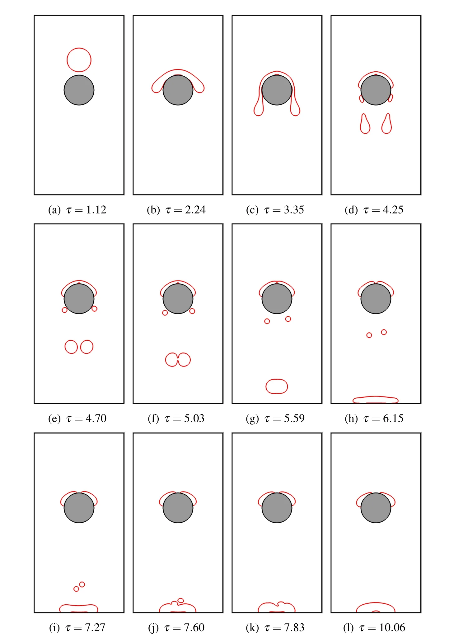
Figure 13:Shapes of the drop when impacting on the solid with Re=14.1,Eo=12.8.
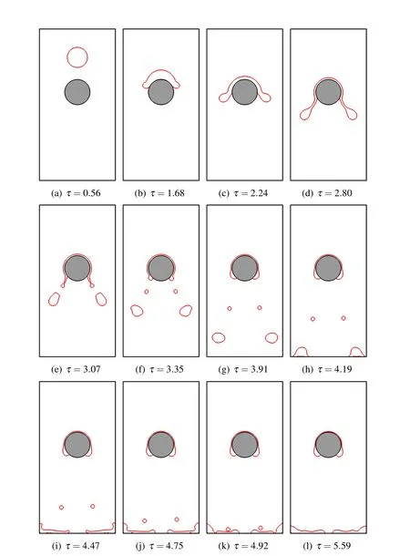
Figure 14:Shapes of the drop when impaction on the solid with Re=141,Eo=12.8.

The values of gravity and surface tension force are manipulated so that two Reynolds number cases withEo=12.8 are studied:1)Re=14.1;2)Re=141.The equilibrium contact angle for both cases is set to be 90?.The advancing and receding angles(θA,θR)are set as(100?,80?),respectively.
Figs.13 and 14 show the drop shapes at different non-dimensional times for case 1 and case 2,respectively.Due to gravity,the drop falls and impacts onto a round obstacle.When the drop is close enough to the solid surface,the points-regeneration scheme helps form the contact line by connecting the interfacial points to the solid obstacle(Figs.13(b)and 14(b)).Then the movement of the contact line conforms to the dynamic contact line model(using Eq.(16))and the given surface hysteresis.For case 1 that has a relatively small Reynolds number,the drop tends to drip down(Fig.13(c)).When the surface tension force can no longer be balanced with the gravity of the drips,the drop breaks up into small ones.As shown in Fig.13,the drop undergoes two stages of breaking-up and forms two large drops and two small ones(Fig.13(d)).The two large drops coalesce during falling(Fig.13(f))and eventually impact on the bottom surface and form a round cap(Fig.13(h)).Due to the accumulative precision error,the small drops are not formed at the exact same time.Both of them eventually merge with the two large drops.In case 2 where the Reynolds number is 141,as shown in Fig.14,a different scenario happens.The original drop hits the round obstacle with a larger impact velocity.Therefore the impact is much more dramatic compared to the low Reynolds number case.The drop breaks up into small ones that slash around.Instead of forming a round cap at the bottom surface,the topology of the interface changes constantly.It even climbs onto the side walls during the spreading of these broken drops.
4 Conclusions
In this work,we propose and set up a numerical framework to model drop spreading and impact by coupling a connectivity-free front tracking(CFFT)method with a dynamic contact line model with surface hysteresis.This numerical method can be used as a tool to perform bloodstain pattern analysis as it aims at accurately predicting the drop behaviors such as motion,impact and spreading under gravity,viscosity and surface tension force.The CFFT method explicitly represents the interface using interfacial points without the need to maintain the connectivities.Therefore,the topology change can be easily handled for blood drop spattering.In order to provide more accurate simulation for contact line problem,we adopt a macroscopic dynamic contact line model to predict the contact angle.This model is implemented by reconstructing the contact region of the air-liquid interface to adjust the actual geometrical contact angle according to the model prediction.With the explicit interfacial points representation,the reconstruction is accurately performed and the dynamic contact angle constraint is successfully imposed.
Several test cases are shown to validate the method.In the drop spreading due to gravity case,the normalized maximum height of the drop agrees very well with the theoretical prediction.By performing the drop movement on an oblique surface case,we find the critical angles of the oblique surface with variousEonumber and surface hysteresis to match well with the theoretical ones,and numerical results of the receding angles for the inclined drop agree with the experimental data.Finally,the method is applied to a more complicated case by impacting the drop onto a solid obstacle.The drop undergoes frequent interface topology changes.The formation and movement of the contact lines when the drop interacts with solid surfaces are well presented.The results show the different behaviors of the drop due to different Reynolds numbers hence the impact velocities,which indicates great flexibility and robustness of the method.
We acknowledge that the implementation as well as the test cases were limited to 2-D at this point due to the complex and heavy computational cost involved in constructing 3-D surfaces without interfacial connectivity.However,this work is to demonstrate the applicability in accurately modeling drop spreading and impact problems that are not trivial in many numerical aspects.To our knowledge,this is a first attempt in combining a connectivity-free multiphase approach with a dynamic contact line model,which shows great promises in building a robust numerical framework to be widely adopted in BPA and forensic science.
Afkhami,S.;Zaleski,S.;Bussmann,M.(2009):A mesh-dependent model for applying dynamic contact angles to vof simulations.Journal of Computational Physics,vol.207,pp.5370–5389.
Attinger,D.;Moore,C.;Donaldson,A.;Jafari,A.;Stone,H.A.(2013):Fluid dynamics topics in bloodstain pattern analysis:Comparative review and research opportunities.Forensic Science International,vol.231,no.1-3,pp.375–396.
Brackbill,J.U.;Kothe,D.B.;Zemach,C.(1992): A continuum method for modeling surface tension.Journal of Computational Physics,vol.100,pp.335–354.
Cervone,A.;Manservisi,S.;Scardovelli,R.(2010):Simulation of axisymmetric jets with a finite element Navier-Stokes solver and a multilevel VOF approach.Journal of Computational Physics,vol.229,no.19,pp.6853–6873.
Chen,Y.;Mertz,R.;Kulenovic,R.(2009): Numerical simulation of bubble formation on orifice plates with moving contact line.International Journal of Multiphase Flow,vol.35,pp.66–77.
Di,Y.;Wang,X.(2009):Precursor simulations in spreading using a multi-mesh adaptive finite element method.Journal of Computational Physics,vol.228,pp.1380–1390.
Dupont,J.-B.;Legendre,D.(2010):Numerical simulation of static and slideing drop with contact angle hysteresis.Journal of Computational Physics,vol.229,pp.2453–2478.
ElSherbini,A.;Jacobi,A.(2006):Retention forces and contact angles for critical liquid drops on non-horizontal surfaces.Journal of Colloid and Interface Science,vol.299,pp.841–849.
Herrmann,M.(2008): A balanced force refined level set grid method for twophase flows on unstructured flow solver grids.Journal of Computational Physics,vol.227,no.4,pp.2674–2706.
Hirt,C.;Nichols,B.(1981):Volume of fluid(vof)method for the dynamics of free boundaries.Journal of Computational Physics,vol.39,no.1,pp.201–225.
Hua,J.;Stene,J.F.;Lin,P.(2008):Numerical simulation of 3d bubbles rising in viscous liquids using a front tracking method.Journal of Computational Physics,vol.227,pp.3358–3382.
Karger,B.;Rand,S.;Fracasso,T.;Pfeiffer,H.(2008): Bloodstain pattern analysis-casework experience.Forensic Science International,vol.181,no.1-3,pp.15–20.
Kistler,S.(1993): Hydrodynamics of wetting.In Berg,J.(Ed):Wettability,pp.311–429,New York.Marcel Dekker.
Liu,W.K.;Jun,S.;Li,S.;Adee,J.;Belytschko,T.(1995):Reproducing kernel particle methods for structural dynamics.International Journal for Numerical Methods in Engineering,vol.38,pp.1655–1679.
Liu,W.K.;Jun,S.;Zhang,Y.F.(1995):Reproducing kernel particle methods.International Journal for Numerical Methods in Fluids,vol.20,pp.1081–1106.
Mukherjee,S.;Abraham,J.(2007):Investigations of drop impact on dry walls with a lattice-baltzmann model.Journal of Colloid and Interface Science,vol.312,pp.341–354.
Muradoglu,M.;Tasoglu,S.(2010):A front-tracking method for computational modeling of impact and spreading of viscous droplets on solid walls.Computers&Fluids,vol.39,pp.615–625.
Muradoglu,M.;Tryggvason,G.(2008): A front-tracking method for computation of interfacial flows with soluble surfactants.Journal of Computational Physics,vol.227,no.4,pp.2238–2262.
Roisman,I.;Opfer,L.;Tropea,C.;Raessi,M.;Mostaghimi,J.;Chandra,S.(2008): Drop impact onto a dry surface:Role of the dynamic contact angle.Colloids and Surfaces A:Physicochemical and Engineering Aspects,vol.322,pp.183–191.
Shi,Y.;Bao,K.;Wang,X.-P.(2013): 3d adaptive finite element method for a phase field model for the moving contact line problems.Inverse Problems and Imaging,vol.7,no.3,pp.947–959.
Sikalo,S.;Wihelm,H.-D.;Roisman,I.(2005): Dynamic contact angle of spreading droplets:Experiments and simulations.Physics of Fluids,vol.17,pp.615–625.
Spelt,P.D.(2005): A level-set approach for simulations of flows with multiple moving contact lines with hysteresis.Journal of Computational Physics,vol.207,pp.389–404.
Tryggvason,G.;Bunner,B.;Esmaeeli,A.;Juric,D.;Al-Rawahi,N.;Tauber,W.;Han,J.;Nas,S.;Jan,Y.-J.(2001):A front-tracking method for the computations of multiphase flow.Journal of Computational Physics,vol.169,no.2,pp.708–759.
Unverdi,S.O.;Tryggvason,G.(1992): A front-tracking method for viscous,incompressible,multi- fluid flows.Journal of Computational Physics,vol.10,pp.25–37.
Wang,C.;Wang,X.;Zhang,L.(2013):Connectivity-free front tracking method for multiphase flows with free surfaces.Journal of Computational Physics,vol.241,pp.58–75.
Witteveen,J.;Koren,B.;Bakker,P.(2007):An improved front tracking method for the euler equations.Journal of Computational Physics,vol.224,no.2,pp.712–728.
Xu,J.-J.;Li,Z.;Lowengrub,J.;Zhao,H.(2006): A level-set method for interfacial flows with surfactant.Journal of Computational Physics,vol.212,no.2,pp.590–616.
 Computer Modeling In Engineering&Sciences2014年7期
- Computer Modeling In Engineering&Sciences的其它文章
- Particle-Based Moving Interface Method for The Study of the Interaction Between Soft Colloid Particles and Immersed Fibrous Network
- A Meshfree Method For Mechanics and Conformational Change of Proteins and Their Assemblies
- Large Deformation Dynamic Three-Dimensional Coupled Finite Element Analysis of Soft Biological Tissues Treated as Biphasic Porous Media
- Preface