Jiaojiao Xiong Hongyang Lu Minghui Zhang Qiegen Liu

1 Introduction

Magnetic resonance imaging(MRI)is a crucial medical diagnostic technique which offers clinicians with signi fi cant anatomical structure for lack of ionizing.Unfortunately,although it enables highly resolution images and distinguishes depiction of soft tissues,the imaging speed is limited by physical and physiological constraints and increasing scan duration may bring in some physiological motion artifacts[1].Therefore,it is necessary to seek for a method to decrease the acquisition time.Reducing the number of measurements mandated by Nyquist sampling theory is a way to accelerate the data acquisition at the expense of introducing aliasing artifacts in the reconstructed results.In recent years,compressed sensing(CS)theory,as a promising method,has proposed an essential theoretical foundation for improving data acquisition speed.Particularly,the application of CS to MRI is known as CS-MRI[2]?[6].

The CS theory states that the image which has a sparse representation in certain domain can be recovered from a reduced set of measurements largely below Nyquist sampling rates[2].The traditional CS-MRI usually utilizes prede fi ned dictionaries[1],[7]?[9],which may fail to sparsely represent the reconstructed images.For instance,Lustiget al.[1]employed the total variation(TV)penalty and the Daubechies wavelet transform for MRI reconstruction.Trzaskoet al.[6]proposed a homotopic minimization strategy to reconstruct the MR image.Instead,adaptive dictionary updating in CS-MRI can provide less reconstruction errors due to the dictionary learned from sampled data[10],[11]. Recently,Ravishankaret al.supposed that each image patch has sparse representation,and presented a prominent two-step alternating method named dictionary learning based MRI reconstruction(DLMRI)[12].The fi rst step is for adaptively learning the dictionary,and the second step is for reconstructing image from undersampledk-space data.Numerical experiments have indicated that these data-driven-learning approaches obtained considerable improvements than previous prede fi ned dictionaries-based methods.Liuet al.[13]proposed a gradient based dictionary learning method for image reconstruction(GradDL),which alleviated the drawback of the popular TV regularization by employing dictionary learning technique.Speci fi cally,it fi rstly trained dictionaries from the horizontal and vertical gradients of the image respectively,and then reconstructed the desired image using the sparse representations of both derivatives.They also extended their ideas to the CT reconstruction and InSAR phase noise fi ltering[14],[15].Nevertheless,most of existing methods did not consider the geometrical pro fi t information sufficiently,which may lead to the fi ne details to be lost.

All the above methods use conventional patch-based sparse representation to reconstruct MR image,it has a fundamental disadvantage that the important spatial structures of the image of interest may be lost due to the subdivision into patches that are independent of each other.To make up for de fi ciencies of conventional patch-based sparse representation method,Zeileret al.[16]proposed a convolutional implementation of sparse coding method(CSC).In the convolutional decomposition procedure,the decomposition does not need to divide the entire image into overlapped patches,and can naturally utilize the consistency prior.CSC was fi rst introduced in the context of modeling receptive fi elds in human vision[17].Recently,it has been demonstrated that CSC has important applications in a wide range of computer vision problems,like low/midlevel feature learning,low-level reconstruction[18],[19],networks in high-level computer vision or hierarchical struc-tures challenges[16],[20],[21],and in physically-motivated computational imaging problems[22],[23].In addition,CSC can fi nd applications in many other reconstruction tasks and feature-based methods,including denoising,inpainting,super-resolution and classi fi cation[24]?[30].

In this paper,we propose a new formulation of convolutional sparse coding tailored to the problem of MRI reconstruction.Moreover,due to the image gradients are a sparser representation than the image itself and therefore may have sparser representation with the CSC than the pixel-domain image,we learn CSC in gradient domain for better quality and efficient reconstruction.The present method has two bene fi ts. First,we introduce CSC for MRI reconstruction.Second,since the image gradients are usually sparser representation than the image itself,it is demonstrated that the CSC in gradient domain could lead to sparser representation than those using the conventional sparse representation methods in the pixel domain.

The remainder of this paper is organized as follows.Section 2 states the prior work in CS and CSC.The proposed algorithm CSC in gradient domain(GradCSC)that employing the augmented Lagrangian(AL)iterative method is detailed in Section 3.Section 4 demonstrates the performance of the proposed algorithm on examples under a variety of sampling schemes and undersampling factors.Conclusions are given in Section 5.

2 Background

In this section,we fi rst review several classical models for CS-MRI,and then introduce the theory of CSC.The following notational conventions are used throughout the paper.Letu∈CNdenotes an image to be reconstructed,andf∈CQrepresents the undersampled Fourier measurements.The partially sampled Fourier encoding matrixFp∈CQ×Nmapsutofsuch thatFpu=f.An MRI reconstruction problem is formulated as the retrieval of the vectorubased on the observationfand given the encoding matrixFp.

2.1 CS-MRI

The choice of sparsifying transform is an important question in CS theory.In the past several years,reconstructing unknown image from undersampled measurements was usually formulated as in(1)where assuming the image gradients are sparse

Sparse and redundant representations of image patches based on learned basis has been drawing considerable attention in recent years.Speci fi cally,Ravishankaret al.[12]presented a method named DLMRI to reconstruct MR image from highly undersampledk-space data with its objective shown as follows:

where Γ =[α1,α1,...,αL]denotes the sparse coefficient matrix of image patches,R(u)=[R1u,R2u,...,RLu]consisting ofLsignals,‖·‖0denotes thel0quasi-norm which counts the number of non-zero coefficients of the vector andT0controls the sparsity of the patch representation.Images are reconstructed by the minimization of a linear combination of two terms corresponding to dictionary learningbased sparse representation and least squares data fi tting.The fi rst term enforces sparsity of the image patches with respect to an adaptive dictionary,and the second term enforces data fi delity ink-space.The method exhibited superior performance compared to those using fi xed basis,through learned adaptive transforms from image.Since DL techniques are more effective and efficient in the sparse domain of the image,Liuet al.[13]proposed a model to reconstruct the image by iteratively reconstructing the gradients via dictionary learning and solving for the fi nal image,instead of learning adaptive structure from the image itself.The method is based on the observation that the gradients are sparser than the image itself.Therefore,it possesses sparser representation in the learned dictionary than the pixel-domain.

Although conventional patch-based sparse representation has widely applications,it has some drawbacks.First,it typically assumes that training image patches are independent from each other,hence the consistency of pixels and important spatial structures of the signal of interest may be lost.This assumption typically results in fi lters are simply translated versions of each other,and generates highly redundant feature representation.Second,due to the nature of the mathematical formulation that a linear combination of learned patches,these traditional patchbased representation approaches may fail to adequately represent high-frequency and high-contrast image features,thus loses some details and textures of the signal,which is important for MR images.

2.2 Convolutional Sparse Coding

Zeileret al.[16]proposed an alternative to patchbased approaches named CSC,decomposing the image into spatially-invariant convolutional features.CSC is the sum of a set of convolutions of the feature maps by replacing the linear combination of a set of dictionary vectors.LetXbe a training set containing 2Dimages with dimensionm×n.Letbe the 2Dconvolutional fi lter bank havingKfi lters,where eachdkis ah×hconvolutional kernel.zkis the sparse feature maps,each of which is the same size asX.CSC aims to decompose the input imageXinto the sparse feature mapszkconvolved with kernelsdkfrom the fi lter bankD,by solving the following objective function:

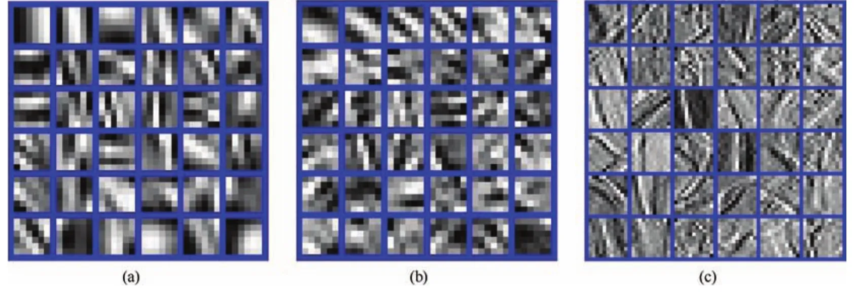
Fig.1. One illustration of fi lters learned.(a)Learned dictionary by DLMRI,(b)Learned dictionary by GradDL,and(c)Learned fi lter by GradCSC,respectively.

where the fi rst and the second terms represent the reconstruction error and the?1-norm penalty respectively;βis a regularization parameter that controls the relative weight of the sparsity term;?is the 2Ddiscrete convolution operator;and fi lters are restricted to have unit energy to avoid trivial solutions.Note that here‖zk‖1represents the entrywise matrix norm,the construction of is realized by balancing the reconstruction error and the?1-norm penalty.

However,the CSC has led to some difficulties in optimization,Zeileet al.[16]used the continuation method to relax the equality constraints,and employed the conjugate gradient(CG)decent to solve the convolutional least square approximation problem.By considering the property of block circulant with circulant block(BCCB)matrix in the Fourier domain,Bristowet al.[32]presented a fast CSC method.Recently,Wohlberg[33]presented an effi-cient alternating direction method of multipliers(ADMM)to further improve this method.

3 Convolutional Sparse Coding in Gradient Domain

The image gradients are sparser than the image itself[13],therefore it has sparser representation in the CSC than that in the pixel-domain image.This motivates us to consider the CSC in the gradient domain.It is expected that such learning is more accurate and robust than that from pixel domain.In this work,we propose an algorithm to reconstruct the image by iteratively reconstructing the gradients via CSC and solving for the fi nal image.

3.1 Proposed Model

To reconstruct image from the image gradients,we propose a new model as follows:

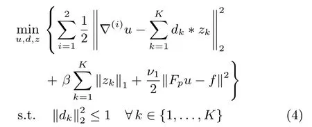
where(▽x,▽y)=(▽(1),▽(2)).The fi rst term and the second term in the cost function(4)capture the sparse prior of the gradient image patches with respect to CSC,and the third termrepresents the data fi delity term ink-space withl2-norm controlling the error.The weightv1balances the tradeoffbetween these three terms,and is set asν1=(λ1/σ)like the DLMRI algorithm does[13],whereλ1is a positive constant.βis a regularization parameter and controls the relative weight of the sparsity term with respect to the data term.The constraint,?k∈{1,...,K}can be included in the objective function via an indicator functionindC(·),which is de fi ned on the convex set of the constraint.

In order to better understand the bene fi t of the CSC in the gradient domain,one demonstration of visual inspection between traditional sparse coded dictionaries and GradCSC fi lter is shown in Fig.1.The learned dictionaries by DLMRI and GradDL are depicted in Figs.1(a)and(b),both of which are learned from the Lumbar spine image in Fig.2.The learned fi lters by GradCSC shown in Fig.1(c)are learned from the dataset in[16].Compared to the traditional sparse coded dictionaries in Figs.1(a)and(b),it can be seen from Fig.1(c)that the convolutional fi lter in GradCSC shows less redundancy,crisper features,and a larger range of feature orientations.

3.2 Algorithm Solver

In the regularization term of(4),the global fi nite difference operators▽(i)are coupled,hence we resort to the splitting technique to decouple them.Speci fi cally,to fi nd a solution to the model(4),an AL iterative technique is employed and an algorithm called GradCSC is developed.The algorithm alternately updates sparse representations of the image patches,reconstructs the horizontal and vertical gradients,and estimates the original image from both gradients.A full description of the algorithm is given in Algorithm 1.

Equation(4)can be rewritten as follows by introducing auxiliary variablesw(i),i=1,2.

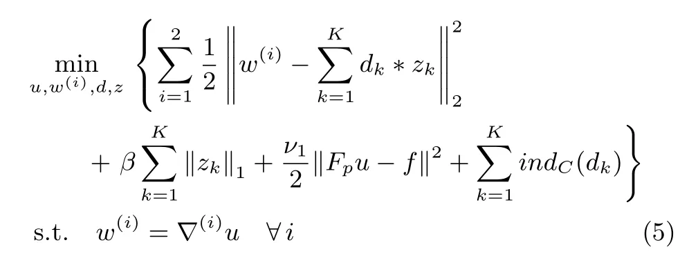
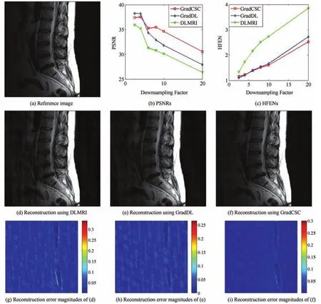
Fig.2. The reconstruction results of the Lumbar spine image under different undersampling factors with 2D random sampling.

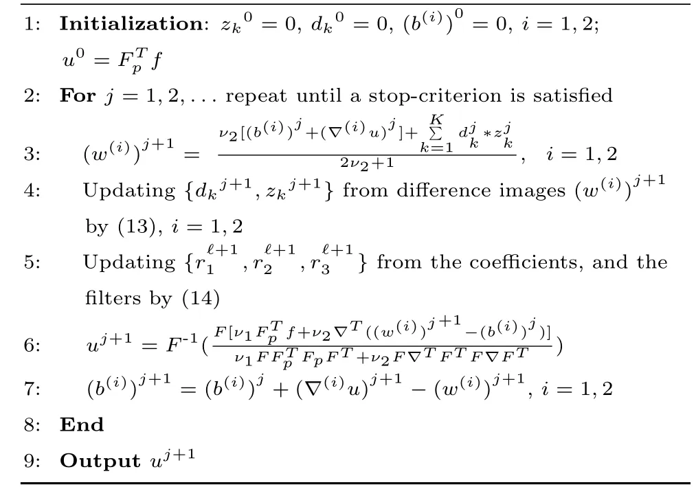
Algorithm 1.The GradCSC algorithm

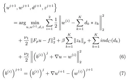
whereν2denotes the positive penalty parameter. The ADMM can be used to address the minimization of(6)with respect tou,w,z,andd.This technique carries out approximation via alternating minimization with respect to one variable while keeping other variables fi xed.

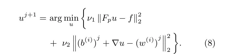
1)Updating the Solution u:At thejth iteration,we assumew,z,anddto be fi xed with their values denoted aswj,zj,anddj,respectively.Eliminating the constant variables,the objective function for updatinguis given as

Recognizing that(8)is a simple least squares problem admitting an analytical solution.The least squares solution satis fi es the normal equation

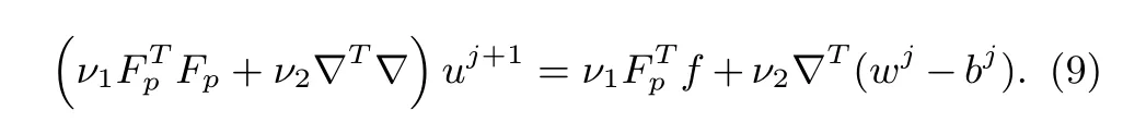
However,directly solving the equation can be tedious due to(9)has a high computation complexity(O(P3)).Fortunately,we can use the convolution theorem of Fourier transform to obtain the solution:

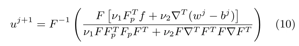
similarly as described in DLMRI and GradDL method[12],the matrixis a diagonal matrix consisting of ones and zeroes corresponding to the sampled location ink-space.

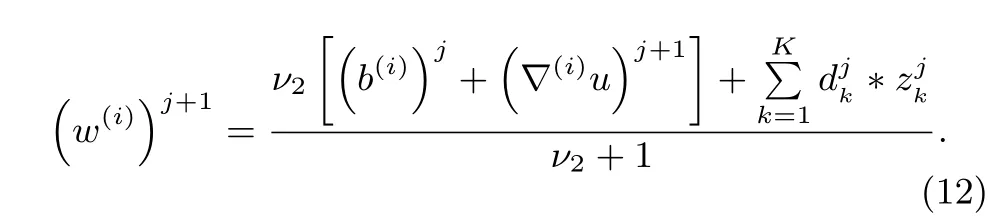
2)Updating the Gradient Image Variables w(i),i=1,2:The minimization in(6)with respect tow(1)andw(2)are decoupled,and then can be solved separately.It yields:

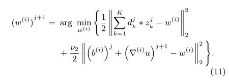
The least squares solution satis fi es the normal equation,and the solution of(11)is as follow:

3)Updating the Coefficients z,and the Filters d:The minimization(6)with respect to CSC and coefficient variables of the gradient image in horizontal and vertical yields:

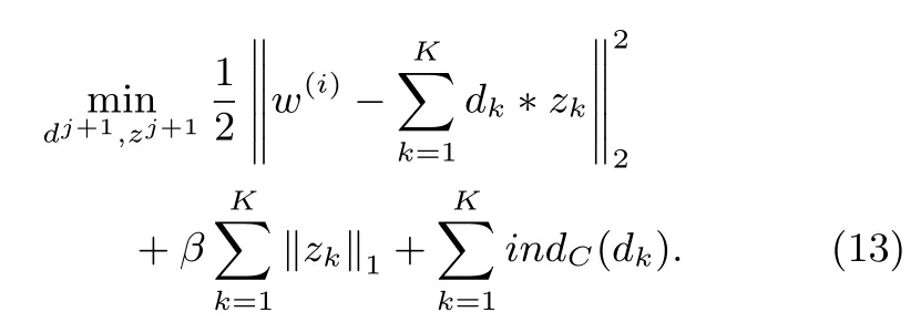
The problem in(13)can be solved by employing an AL algorithm like mentioned above,(13)needs to introduce auxiliary variables,it solves:

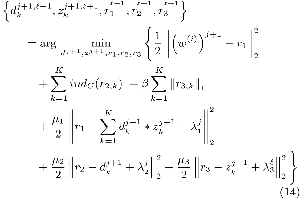
at the?th iteration fordj+1,?+1,zj+1,?+1,then updates the multipliersλ1,λ2andλ3by the formula

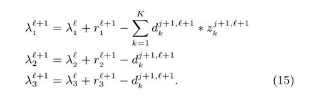
ADMM is chosen to solve the(14).The corresponding fi ve subproblems can be solved as follows:

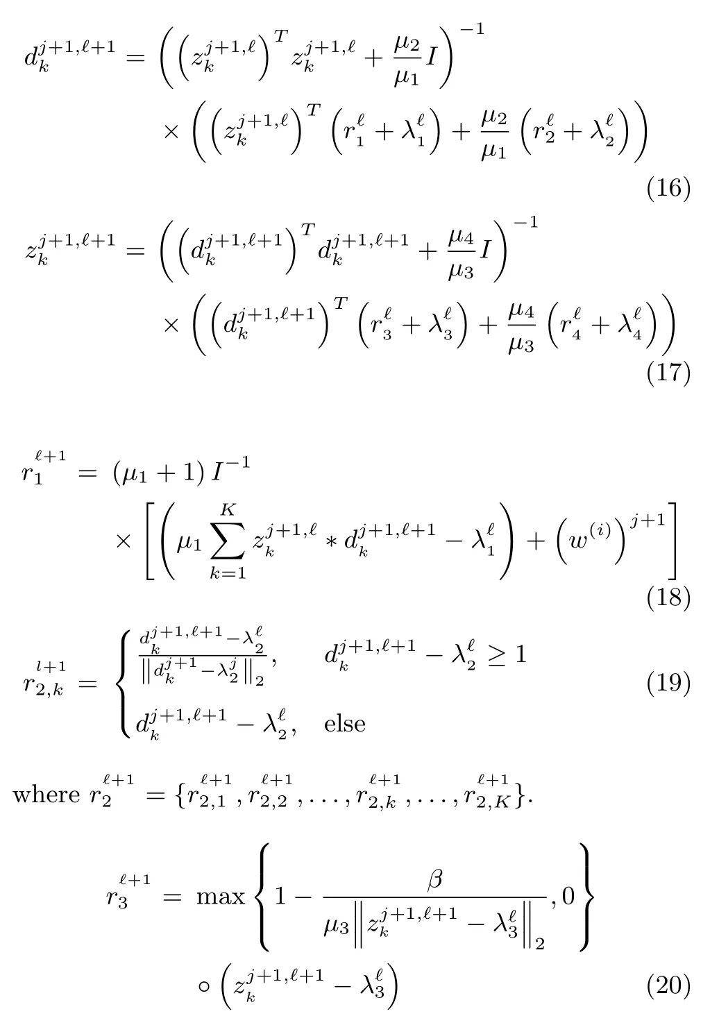
where?represents the point-wise product function and the operation is implemented by component-wise manner.

4 Experimental Results

In this section,we evaluate the performance of proposed method at a variety of sampling schemes and undersampling factors.The sampling schemes employed in the experiments contain the 2D random sampling,pseudo radial sampling,and Cartesian sampling with random phase encoding(1D random).The size of images we use in the synthetic experiments are 512×512.The CS data acquisition was simulated by subsampling the 2D discrete Fourier transform of the MR images(except the test with real acquired data)in the light of many prior work on CS-MRI approaches,.In order to fi nd the sparse feature mapzk,we use a fi xed fi lterDwhich is trained from reference MR images.We fi nd that learningK=100 fi lters of size 11×11 pixels ful fi lls these conditions for our data and works well for all the images tested.In the experiment,the proposed method GradCSC is compared with the leading DLMRI[12]and GradDL[13]methods that have shown the substantially outperform other CS-MRI methods.In addition,we use the peak signal-to-noise ratio(PSNR)and highfrequency error norm(HFEN)[20]to evaluate the quality of reconstruction.All of these algorithms are implemented in MATLAB 7.1 on a PC equipped with AMD 2.31GHz CPU and 3GByte RAM.

4.1 Experiments Under Different Undersampling Factors

In this subsection,we evaluate the performance of Grad-CSC under different undersampling factors with same sampling scheme.Fig.2 illustrates the reconstruction results at a range of undersampling factors with 2.5,4,6,8,10 and 20.We added the zero-mean complex white Gaussian noise withσ=10.2 in the 2D random sampledk-space.The PSNR and HFEN values for DLMRI,GradDL and GradCSC at various undersampling factors are presented in Figs.2(b)and(c),additionally the PSNR values are listed in Table I.For the subjective comparison,the construction results and magnitude image of the reconstruction error provided by the three methods at 8-fold undersampling are presented in Figs.2(d),(e),(f)and(g),(h),(i),respectively.In this case,it can be seen that the image reconstructed by the DLMRI method(shown in Fig.2(d))is blurred and loses some textures.Although both GradDL and GradCSC present excellent performances on suppressing aliasing artifacts,our GradCSC provides a better reconstruction of object edges(such as the spine)and preserves fi ner texture information(such as the bottom-right of the reconstruction).Such difference in reconstruction quality is particularly clear in the image errors shown in Figs.2(g),(h)and(i).In general,our proposed method provides greater intensity fi delity to the image reconstructed from the full data.

4.2 Impact of Undersampling Schemes

In this subsection,we evaluate the performance of Grad-CSC at various sampling schemes.The results are presented in Fig.3 which reconstructed an axial T2-weighted brain image at 8-fold undersampling factors by applying three different sampling schemes,including 2D random sampling,1D Cartesian sampling,and pseudo radial sampling.The PSNR and HFEN indexes versus iterative number for method DLMRI,GradDL and GradCSC are plotted in Figs.3(b)and(c).Particularly,we present the reconstructions of DLMRI,GradDL and GradCSC with 2D random sampling in Figs.3(d),(e),and(f),respectively.In order to facilitate the observation,the difference image between reconstruction results are shown in Figs.3(g),(h),and(i).As can be expected,the convolution operator enables CSC outperform DLMRI and GradDL methods for most of speci fi ed undersampling ratios and trajectories.This exhibits the bene fi ts of employing the convolutional fi lter for sparse coding. In particular,in Fig.3(d),(e),and(f)the skeletons in the top half part of the Grad-CSC reconstruction appear less obscured than those in the DLMRI and GradDL results.the proposed method Grad-CSC reconstructs the images more accurately with larger PSNR and lower HFEN values than the GradDL approach.Particularly when sampled at 2D random trajectory,our method GradCSC outperforms others with a remarkable improvement from 0.7dB to 5.8dB.

4.3 Performances at Different Noise Levels

We also conduct experiments to investigate the sensitivity of GradCSC to different levels of complex white Gaussian noise.DLMRI,GradDL and GradCSC are applied to reconstruct a noncontrast MRA of the circle of Willis under pseudo radial sampling at 6.67-fold acceleration.Fig.4 presents the reconstruction results of three methods at different levels of complex white Gaussian noise,which are added to thek-space samples.Fig.4(c)presents the PSNRs of DLMRI,GradDL and GradCSC at a sequence of different standard deviations(0,2,5,8,10,12,15).Reconstruction results with noise 5 are shown in Figs.4(d),(e),and(f).The PSNRs gained by DLMRI and GradDL are 27.03dB and 29.78dB,while the GradCSC method achieves 30.45dB.Obviously,the reconstruction obtained by GradCSC is clearer than those by DLMRI and GradDL.It can be observed that our GradCSC method can reconstruct the images more precisely than DLMRI and GradDL,in terms of extracting more structural and detail information from gradient domain.The corresponding error magnitudes of the reconstruction are displayed in Figs.4(g),(h),and(i).It reveals that our method provides a more accurate reconstruction of image contrast and sharper anatomical depiction in noisy case.

5 Conclusion

In this work,a novel CSC method in gradient domain for MR image reconstruction was proposed.The important spatial structures of the signal were preserved by convolutional sparse coding.For the new derived model,we utilized the AL method to implement the algorithm in a few number of iterations.A variety of experimental results demonstrated the superior performance of the method under various sampling trajectories andk-space acceleration factors.The proposed method can produce highly accurate reconstructions for severely undersampled factors.It provided superior performance in both noiseless and noisy cases.The presented framework will be extended to parallel imaging applications in the future work.

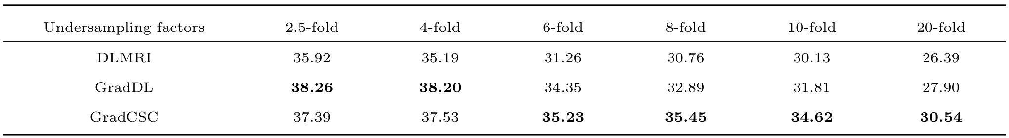
TABLE I RECONSTRUCTION PSNR VALUES AT DIFFERENT UNDERSAMPLING FACTORS WITH THE SAME 2D RANDOM SAMPLING TRAJECTORIES

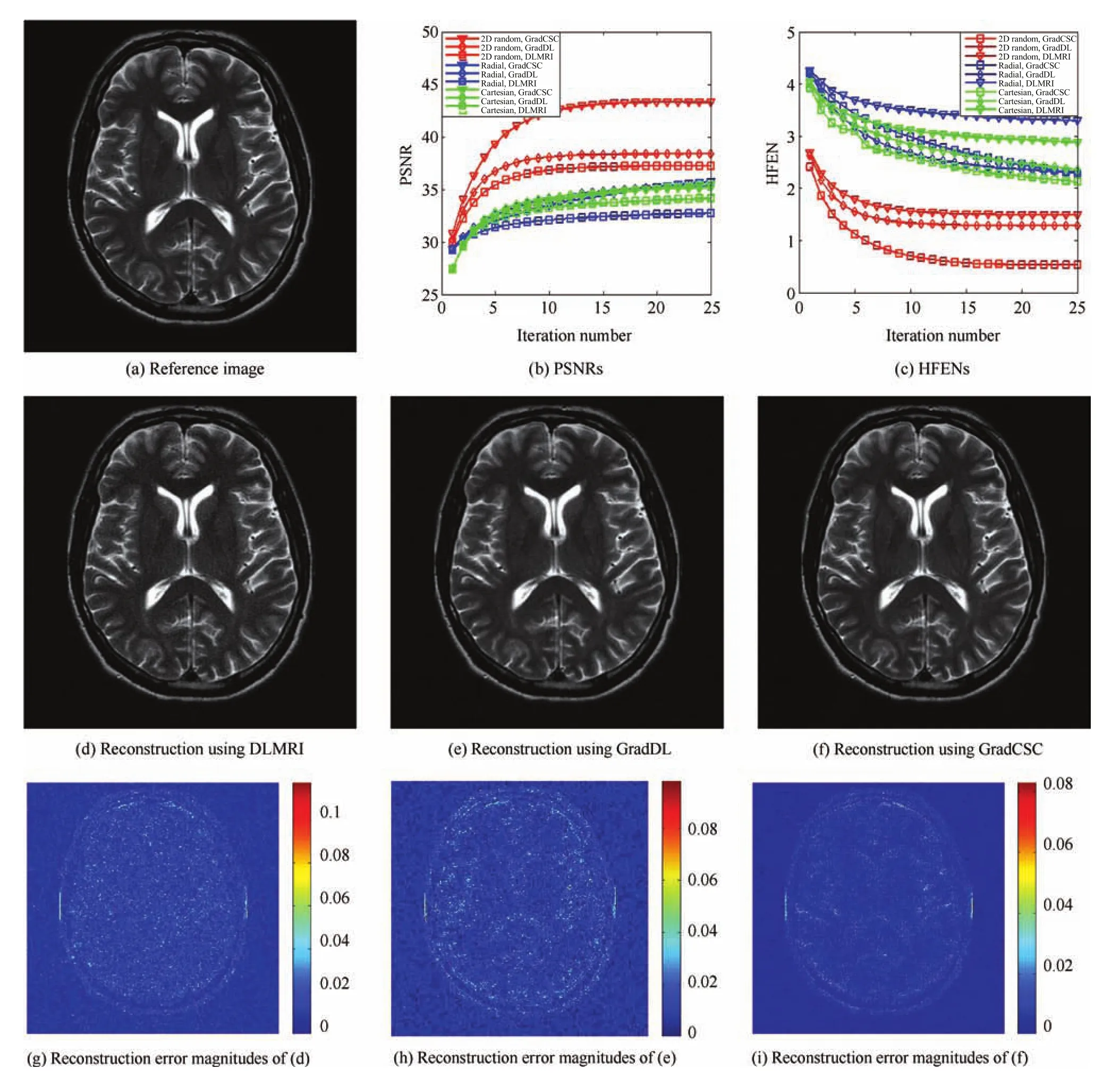
Fig.3.The reconstruction results of the axial T2-weighted brain image under different undersampling schemes.

1 M.Lustig,D.Donoho,and J.M.Pauly,“Sparse MRI:The application of compressed sensing for rapid MR imaging,”Magn.Reson.Med.,vol.58,no.6,pp.1182?1195,Dec.2007.

2 D.L.Donoho,“Compressed sensing,”IEEE Trans.Inform.Theory,vol.52,no.4,pp.1289?1306,Apr.2006.

3 D.Liang,B.Liu,J.Wang,and L.Ying,“Accelerating SENSE using compressed sensing,”Magn.Reson.Med.,vol.62,no.6,pp.1574?1584,Dec.2009.

4 M.Lustig,J.M.Santos,D.L.Donoho,and J.M.Pauly,“k-t SPARSE:high frame rate dynamic MRI exploiting spatiotemporal sparsity,”inProc.13th Ann.Meeting of ISMRM,Seattle,USA,2006.

5 S.Q.Ma,W.T.Yin,Y.Zhang,and A.Chakraborty,“An efficient algorithm for compressed MR imaging using total variation and wavelets,”inProc.IEEE Conf.Computer Vision and Pattern Recognition,Anchorage,AK,USA,2008,pp.1?8.

6 J.Trzasko and A.Manduca,“Highly undersampled magnetic resonance image reconstruction via homotopic?0-minimization,”IEEE Trans.Med.Imaging,vol.28,no.1,pp.106?121,Jan.2009.

7 S.M.Gho,Y.Nam,S.Y.Zho,E.Y.Kim,and D.H.Kim,“Three dimension double inversion recovery gray matter imaging using compressed sensing,”Magn.Reson.Imaging,vol.28,no.10,pp.1395?1402,Dec.2010.

8 M.Guerquin-Kern,M.Haberlin,K.P.Pruessmann,and M.Unser,“A fast wavelet-based reconstruction method for magnetic resonance imaging,”IEEE Trans.Med.Imaging,vol.30,no.9,pp.1649?1660,Sep.2011.

9 L.Y.Chen,M.C.Schabel,and E.V.R.DiBella,“Reconstruction of dynamic contrast enhanced magnetic resonance imaging of the breast with temporal constraints,”Magn.Reson.Imaging,vol.28,no.5,pp.637?645,Jun.2010.

10 Q.G.Liu,S.S.Wang,K.Yang,J.H.Luo,Y.M.Zhu,and D.Liang,“Highly undersampled magnetic resonance image reconstruction using two-level Bregman method with dictionary updating,”IEEE Trans.Med.Imaging,vol.32,no.7,pp.1290?1301,Jul.2013.

11 X.B.Qu,D.Guo,B.D.Ning,Y.K.Hou,Y.L.Lin,S.H.Cai,and Z.Chen,“Undersampled MRI reconstruction with patch-based directional wavelets,”Magn.Reson.Imaging,vol.30,no.7,pp.964?977,Sep.2012.

12 S.Ravishankar and Y.Bresler,“MR image reconstruction from highly undersampled k-space data by dictionary learning,”IEEE Trans.Med.Imaging,vol.30,no.5,pp.1028?1041,May 2011.

13 Q.G.Liu,S.S.Wang,L.Ying,X.Peng,Y.J.Zhu,and D.Liang,“Adaptive dictionary learning in sparse gradient domain for image recovery,”IEEE Trans.Image Process.,vol.22,no.12,pp.4652?4663,Dec.2013.

14 Z.L.Hu,Q.G.Liu,N.Zhang,Y.W.Zhang,X.Peng,P.Z.Wu,H.R.Zheng,and D.Liang,“Image reconstruction from few-view CT data by gradient-domain dictionary learning,”J.X-Ray Sci.Technol.,vol.24,no.4,pp.627?638,Jul.2016.

15 X.M.Luo,Z.Y.Suo,and Q.G.Liu,“Efficient InSAR phase noise fi ltering based on adaptive dictionary learning in gradient vector domain,”Chin.J.Eng.Math.,vol.32,no.6,pp.801?811,Dec.2015.

16 M.D.Zeiler,D.Krishnan,G.W.Taylor,and R.Fergus,“Deconvolutional networks,”inProc.2010 IEEE Conf.Computer Vision and Pattern Recognition(CVPR),San Francisco,CA,USA,2010,pp.2528?2535.

17 B.A.Olshausen and D.J.Field,“Sparse coding with an overcomplete basis set:a strategy employed by V1?,”Vision Res.,vol.37,no.23,pp.3311?3325,Dec.1997.

18 A.Szlam,K.Kavukcuoglu,and Y.LeCun,“Convolutional matching pursuit and dictionary training,”arXiv:1010.0422,Oct.2010.

19 B.Chen,G.Polatkan,G.Sapiro,D.Blei,D.Dunson,and L.Carin,“Deep learning with hierarchical convolutional factor analysis,”IEEE Trans.Pattern Anal.Mach.Intell.,vol.35,no.8,pp.1887?1901,Aug.2013.

20 K.Kavukcuoglu,P.Sermanet,Y.L.Boureau,K.Gregor,M.Mathieu,and Y.LeCun,“Learning convolutional feature hierarchies for visual recognition,”inProc.23rd Int.Conf.Neural Information Processing Systems,Vancouver,British Columbia,Canada,2010,pp.1090?1098.

21 M.D.Zeiler,G.W.Taylor,and R.Fergus,“Adaptive deconvolutional networks for mid and high level feature learning,”inProc.2011 IEEE Int.Conf.Computer Vision(ICCV),Barcelona,USA,2011,pp.2018?2025.

22 F.Heide,L.Xiao,A.Kolb,M.B.Hullin,and W.Heidrich,“Imaging in scattering media using correlation image sensors and sparse convolutional coding,”O(jiān)pt.Express,vol.22,no.21,pp.26338?26350,Oct.2014.

23 X.M.Hu,Y.Deng,X.Lin,J.L.Suo,Q.H.Dai,C.Barsi,and R.Raskar,“Robust and accurate transient light transport decomposition via convolutional sparse coding,”O(jiān)pt.Lett.,vol.39,no.11,pp.3177?3180,Jun.2014.

24 J.Y.Xie,L.L.Xu,and E.H.Chen,“Image denoising and inpainting with deep neural networks,”inProc.25th Int.Conf.Neural Information Processing Systems,Lake Tahoe,Nevada,USA,2012,pp.341?349.

25 S.H.Gu,W.M.Zuo,Q.Xie,D.Y.Meng,X.C.Feng,and L.Zhang,“Convolutional sparse coding for image superresolution,”inProc.2015 IEEE Int.Conf.Computer Vision(ICCV),Santiago,Chile,2015,pp.1823?1831.

26 A.Krizhevsky,I.Sutskever,and G.E.Hinton,“Imagenet classi fi cation with deep convolutional neural networks,”inProc.25th Int.Conf.Neural Information Processing Systems,Lake Tahoe,Nevada,USA,2012,pp.1097?1105.

27 Y.Y.Zhu,M.Cox,and S.Lucey,“3D motion reconstruction for real-world camera motion,”inProc.2011 IEEE Conf.Computer Vision and Pattern Recognition(CVPR),Providence,RI,USA,2011,pp.1?8.

28 Y.Y.Zhu and S.Lucey,“Convolutional sparse coding for trajectory reconstruction,”IEEE Trans.Pattern Anal.Mach.Intell.,vol.37,no.3,pp.529?540,Mar.2015.

29 Y.Y.Zhu,D.Huang,F.De La Torre,and S.Lucey,“Complex non-rigid motion 3D reconstruction by union of subspaces,”inProc.2014 IEEE Conf.Computer Vision and Pattern Recognition(CVPR),Columbus,OH,USA,2014,pp.1542?1549.

30 A.Serrano,F.Heide,D.Gutierrez,G.Wetzstein,and B.Masia,“Convolutional sparse coding for high dynamic range imaging,”Computer Graphics,vol.35,no.2,pp.153?163,May 2016.

31 J.F.Yang,Y.Zhang,and W.T.Yin,“A fast alternating direction method for TVL1-L2 signal reconstruction from partial Fourier data,”IEEE J.Sel.Topics Signal Process.,vol.4,no.2,pp.288?297,Apr.2010.

32 H.Bristow,A.Eriksson,and S.Lucey,“Fast convolutional sparse coding,”inProc.2013 IEEE Conf.Computer Vision and Pattern Recognition(CVPR),Portland,OR,USA,2013,pp.391?398.

33 B.Wohlberg, “Efficient convolutional sparse coding,” inProc.2014 IEEE Int.Conf.Acoustics,Speech and Signal Processing(ICASSP),Florence,Italy,2014,pp.7173?7177.