
A Type D Non-Vacuum Spacetime with Causality Violating Curves,and Its Physical Interpretation
2017-05-09 11:46:21FaizuddinAhmed
Faizuddin Ahmed
Ajmal College of Arts and Science,Dhubri-783324,Assam,India
1 Introduction
The Einstein field equations of Genereal Relativity are the set of non-linear partial differential equations whose exact solution is very hard.Some well-known solutions of the field equations admit Closed Causal Curves(CCCs)in the form of closed timelike curves(CTCs),closed timelike geodesics(CTGs)and closed null geodesics(CNGs).The presence of such curves in a spacetime violates the causality condition.Examples of these spacetime are the Godel’s Cosmological solution,[1]van Stockum solution,[2]Tipler’s rotating cylinder,[3]traversable wormholes,[4?5]and the wrap dripe models[6?7]violate the weak energy condition (WEC),Gott’s solution,[8]Krasnikov spacetime,[9]electrovac spacetime,[10]and pure radiation field spacetimes[11?14]have CTCs.Some well-known vacuum spacetimes such as the Kerr and Kerr–Newmann black holes solution[15?16](see also Ref.[17]),NUT-Taub metric,[18]Bonnor metric,[19?20]Ori metric,[21]locally isometric AdS metric,[22]and type N Einstein spacetime[23]have CTCs.In addition.some other CTC spacetime possesses a naked singularity(e.g.Refs.[24]–[27]).Hawking proposed a Chronology Protection Conjecture,[28]which states that the laws of physics will always prevent a spacetime to form CTCs.However,the general proof of Chronology protection conjecture has not yet existed.
2 The Spacetime with Divergence-Free Curvature
Consider the following line element in(t,x,y,z)coordinates

whereα0>0 is a real number.The metric is topologically trivial,and the ranges of the coordinates are

The metric has signature(?,+,+,+)and the determinant of the corresponding metric tensorgμνis

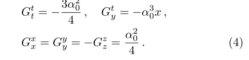
which is regular everywhere even atx=0.The non-zero components of the Einstein tensorGμνare
The scalar curvature invariants of the spacetime
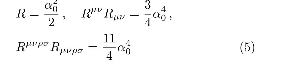
are non-vanishing constant. Therefore,the presented spacetime is free from curvature divergence.
2.1 Stress-Energy Tensor and the Kinematic Parameters
We consider the stress-energy tensor anisotropic fluid for the metric(1)given by
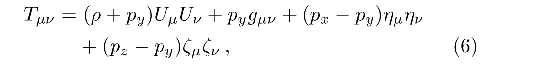
whereρa(bǔ)s the energy density,px,py,andpzare pressures.HereUμis the timelike unit four-velocity vector,ημandζμare the spacelike unit vector alongxandzdirection,respectively.For the metric(1),these are de fined by
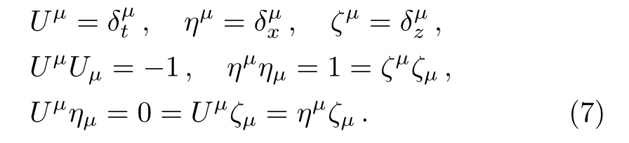
The non-zero components of the stress-energy tensor Eq.(6)using Eq.(7)are
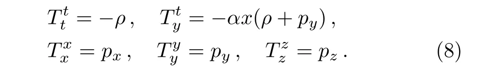
And its trace is given by

The Einstein’s field equations(taking cosmological constant Λ=0)are given by

whereGμνis the Einstein tensor.Here units are chosen such thatc=1 and 8π G=1.Equating the field equations(10)using Eqs.(4)and(8)we get
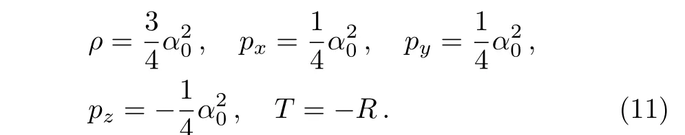
The matter-energy source satisfy the different energy conditions.[17]
The above stress-energy tensor may be a generalization of Equation-of-State(EoS)parameter of perfect fluid by taking EoS parameter separately on each spatial axis.The stress-energy tensor of perfect fluid is given by

We parametrize it as follows:
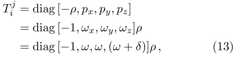
whereωx,ωy,andωzare the directional EoS parameters along thex,y,andzaxis,respectively.Hereωis the deviation-free EoS parameter of the perfect fluid.We have parameterized the deviation from isotropy by settingωx=ω,ωy=ω,and then introducing skewness parameterδthat is the deviation fromωalong thez.
From the stress-energy tensor form(13)using Eq.(11),one will get the Equation-of-state as radiation type
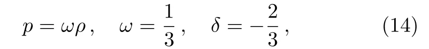
wherepas the isotropic pressure of the fluid.Therefore,our stress-energy tensor is a generalization of Equationof-State(EoS)parameter of perfect fluid(radiation type),whereω=1/3 is the deviation-free EoS parameter andδ=?2/3 is the deviation parameter from isotropy along thez-direction.
The kinematic parameters,the expansion Θ,the acceleration vector˙Uμ,the shear tensorσμν,and the vorticity tensorωμνassociated with the fluid four velocity-vector are de fined by
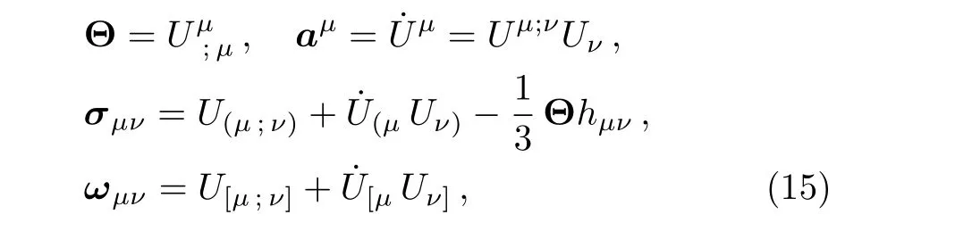
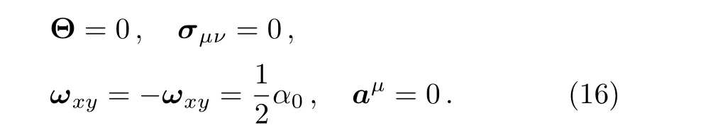
wherehμν=gμν+UμUνis the projection tensor.For the spacetime(1),these parameters have the following expression
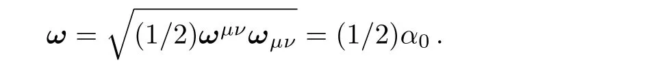
The magnitude of vorticity tensor isωμν,
3 Closed Timelike Curves of the Spacetime
The presented spacetime admit circular closed timelike curves,which appears beyond the null curve.
Consider a closed curveγde fined byt=t0,x=x0,andz=z0,wheret0,x0,z0are constants.Here theycoordinate is chosen periodic,that is eachyidenti fiedy+y0for a certain parametery0>0(see Ref.[21]).From the metric(1),we get

These curves are null curve provided ds2=0 forx2=x20,spacelike provided ds2>0 forx2<x20,but become timelike provided ds2<0 forx2>x20.Therefore,the closed curves de fined byt=t0,x=x0,andz=z0being timelike,are closed timelike curves.Thus the formation of closed timelike curves take places beyond the null curve,i.e.,in the region satisfyingx2>x20,wherex20=1/α20.These curves evolve from an initial spacelike hypersurface.For that we calculate the norm of the vector?μt(or by determining the sign of the componentgttin the metric tensorgμν).[14]From the metric(1),we get

A hypersurfacet=const is spacelike providedgtt<0 forx2<x20,but become timelike providedgtt>0 forx2>x20,and null curvesx2=x20serve as the Chronology horizon.Thus,spaceliket=const.hypersurface can be choosen as initial conditions over which the initial data may be speci fied.Therefore,the formation of closed timelike curves here is identical to the metric in Refs.[1,11,14].
3.1 Stability of Closed Timelike Curves
To analyze the stability of the above closed timelike curves,we used the method adopted in Refs.[11,13–14,29].The closed timelike curves considered here have the parametric form

wheret0,x?,z0are constants.
A CTCγsatis fies the system of equations
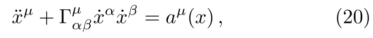
where the dot indicates derivative w.r.t.proper time andaμis a four acceleration.
We consider a small perturbationˉxμ=xμ+ξμin Eq.(20).After perturbation of the system of equations,one can obtain a set of differential equation satis fied by the perturbationξ.We find that
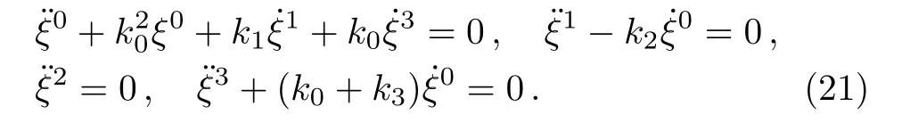
Herek0=α0˙y,k1=2α20x?˙y=2nk0,k2=α20x?˙y=nk0=k1/2,k3=α30x2?˙y=n2k0,andx?=n/α0,wheren>1.
The set of differential equations above can be solved exactly and we obtain the following set of solutions
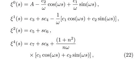
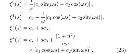
whereci,i=1,...,8 are constants of integration,andω=nk0.The above solutions satisfy the differential equations(21)providedA=?(2n2/ω)c4.For simplicity,we have chosen herec4=0 so thatA=0.Therefore,the set of solutions are
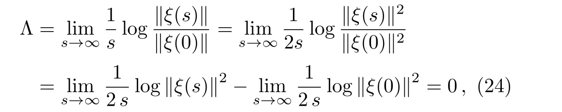
To establish the stability of these orbits(23),one can calculate the largest invariant Lyapunov exponent,a measure of stability of these curves,which we discussed in Refs.[11,13–14].In our case here,we find the Lyapunov exponent de fined by

3.2 Parametric Curves of the Metric:Closed Timelike Curves
For the metric(1),we choose two set of parametric curves de fined by

whereci,fi,i=1,...,8 are arbitrary constants.Taking norm of the tangent vector de fined bygμν(dxμ/ds)(dxν/ds)for the parametric curves(25)using the metric(1),we get a

timelike tangent vector,where we have takenc3=5,c4=c2=1,c6=1,c8=1,α0=1,b=1.We plot a graph of the normgμν(dxμ/ds)(dxν/ds)(vertical axis)w.r.t.s(horizontal axis)shown in Fig.1(a).
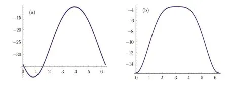
Fig.1 Timelike tangent vector.
Similarly,taking norm of the tangent vector for the parametric curves(26),one will get
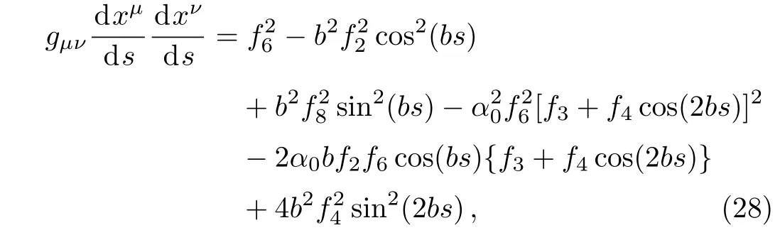
a timelike tangent vector field,where we have takenf3=3,f4=0.1,f2=1,f6=1,f8=1,α0=1,b=1.Ploting a graph of this norm(vertical axis)w.r.t.s(horizontal axis)is shown in Fig.1(b).
Moreover,one can easily show that the above parametric curves are closed in the ranges=0 tos=2π,i.e.,

wherec6=1=f6.Therefore,the parametric curves defined by Eqs.(25)–(26)being timelike and closed,form closed timelike curves(CTCs).
4 Null Geodesics of the Spacetime
In addition to closed timelike curves,the presented spacetime admits null geodesics,which we discuss below.
The spacetime is highly symmetric and admits four Killing vectors in(t,x,y)subspace. These are?t,?y,y?t?(1/α0)?x,(x2?y2)?t+(2/α0)(y?x?x?y).To show that third and fourth are the Killing vector,we take the normal form of these given by
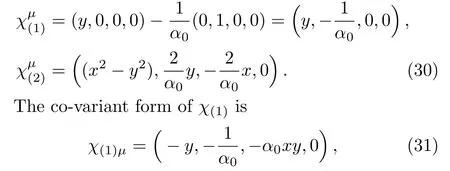
and it satis fies the Killing equation,namely,χ(1)μ;ν+χ(1)ν;μ=0. Similarly,one can show that the vectorχ(2)satis fies the Killing equation.Therefore,the vectors,namely,y?t?(1/α0)?xand(x2?y2)?t+(2/α0)(y?x?x?y)are Killing vector.
The geodesic Lagrangian for the metric(1)is

where we suppresszcoordinate and dot represents derivative w.r.t.λ,an affine parameter.There are two constants of motion corresponding to two cyclic coordinatestandy.These are given by
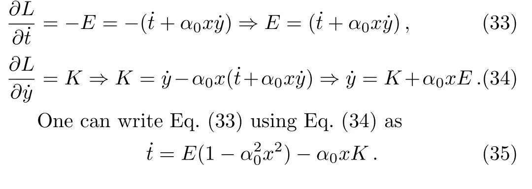
Thus we have,

where ? is the angular velocity with respect to the stationary observers,i.e.,observers moving ont-lines.
If we let the angular momentum about thez-axispy=K=0,we obtain the angular velocity ?0of a ZAMO(zero angular momentum particle as measured by an observer for whomtis the proper time).This is the angular velocity of the frame dragging[30?31]and it is given by

which vanishes,i.e.,?0→0 asx→±∞and changes sign ?0>0 forx2<x20to ?0<0 forx2>x20,wherex20=1/α20.
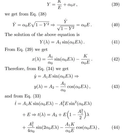
To show the existence of null geodesicL=0 in the spacetime,we first consider the angular momentum is nonzero(K/=0).From Eq.(32)using Eqs.(33)–(34)we get ˙x2+˙y2=(˙t+α0x˙y)2?˙x2=E2?(K+α0xE)2.(38)Writing
whereAi,i=1,...,3 are constants of integration.
Taking norm of the geodesic Eqs.(42)–(44)using the metric(1),we get
gμν˙xμ˙xν=(?1+A21)E2=0,E/=0,(45)a null geodesics condition providedA1=1.The above null geodesics path are closed in the range of the affine parameterλ=0 toλ=1,i.e.,

For non-zero angular momentum,we have the following null geodesics path
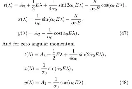
Thus the presented spacetime admits null geodesic with the geodesic equations given by Eq.(47)for non-ZAMO and Eq.(48)for ZAMO(see Fig.2,we have chosenA3=0,α0=1,A2=1,λalong horizontal axis).

Fig.2 (Color online)Null geodesics for ZAMO:blue-t,violet-x,green-y.
5 The Petrov Classi fication of the Spacetime
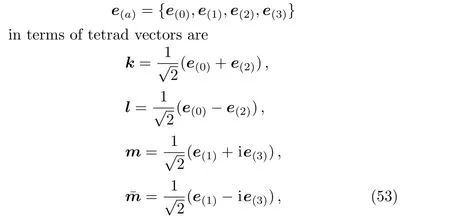
For classi fication of the spacetime(1),we construct the following set of null tetrad vectors(k,l,m,ˉm).[32]They are
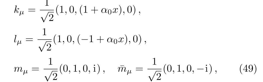
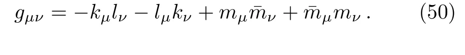
The tetrad vectors(49)are null vectors and are orthogonal except forkμlμ=?1 andmμˉmμ=1.Using the null tetrads above we calculate the five Weyl scalars of which,
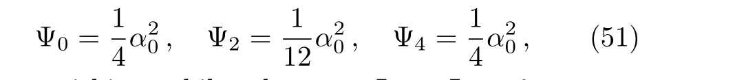
are non-vanishing,while others are Ψ1= Ψ3=0.
One can calculate the Newmann–Penrose spin coefficients[32]using the set of null tetrad vectors(44).We find the nonzero spin-coefficients are
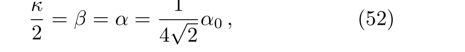
while rest are all equal to zero,where the symbols are same in Ref.[32].
An orthonormal tetrad frame
wheree(0)·e(0)=?1 ande(i)·e(j)=δij.
5.1 The Relative Motion of the Free Test Particles
Here we analyze the effects of the local gravitational fields and the stress-energy tensor terms of the above solutions.For that,we consider the equation of geodesics deviation frame adopted in Refs.[14,26–27].These geodesic equations in terms of orthonormal tetrad are

We set hereZ(0)=0 such that all test particles are synchronized by the proper time.
From the standard de finition of the Weyl tensor we have

For the metric(1),the only non-vanishing Weyl scalars are given by Eq.(49)so that

One can find out the equations of geodesic deviation(54)using Eq.(56)and the stress-energy tensor(6).We
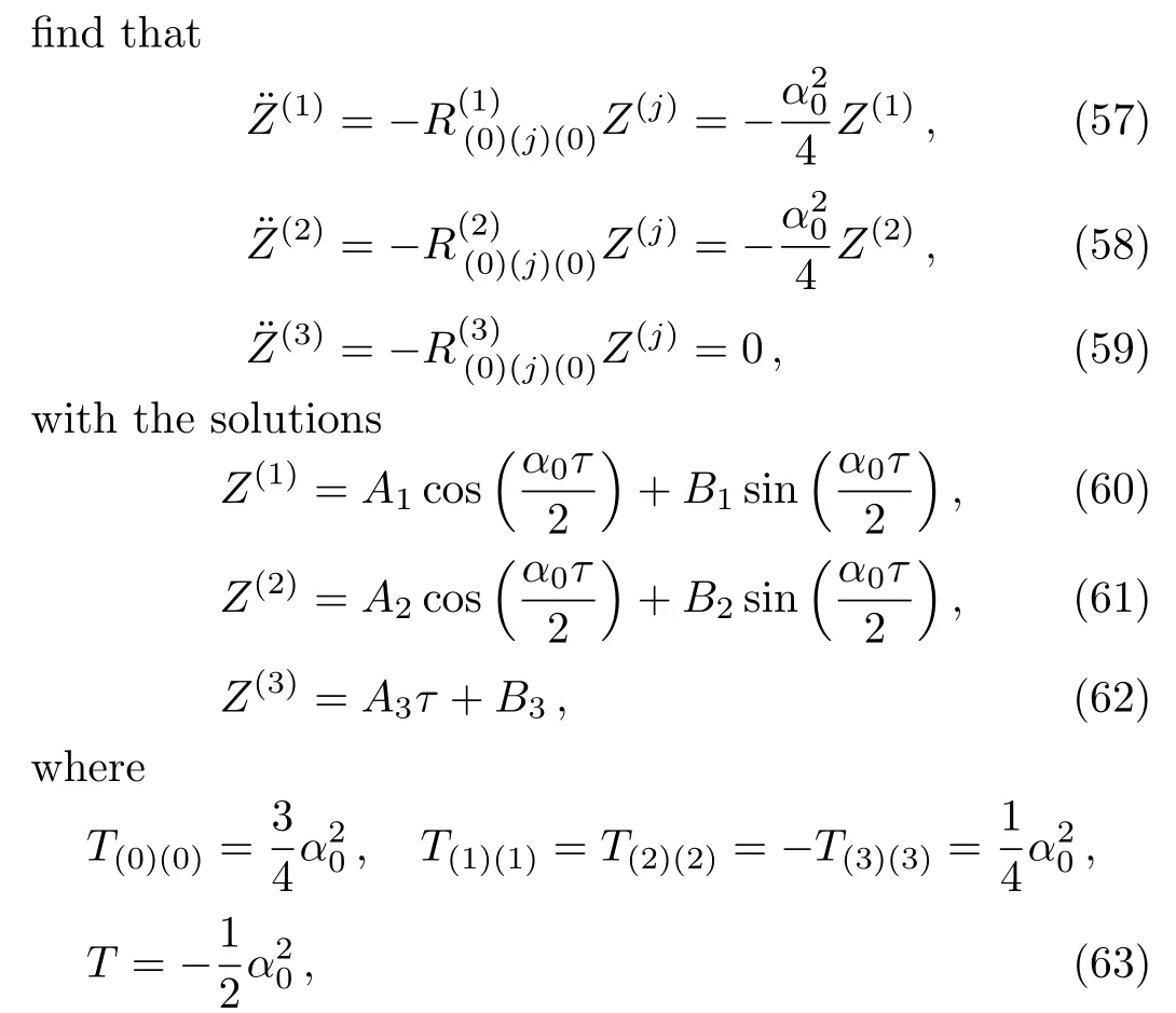
andAi,Bi,i=1,2,3 are arbitrary constants.
6 Conclusions
In this paper,a topologically trivial non-vacuum solution of the Einstein’s field equations,was presented.The spacetime is regular everywhere,and free from curvature divergence since the scalar curvature invariants are constant.The metric admits a twisting,shearfree,nonexpanding timelike geodesic congruence.The physical parameters,the energy densityρ,the radial pressurepr,and the tangential pressureptare constant,which satisfy the different energy conditions.The stress-energy tensor anisotropic fluid considered here is a generalization of Equation-of-State(EoS)parameter of perfect fluidp=ω ρ(radiation type),whereω=1/3 is the deviation-free EoS parameter andδ=?2/3 as the deviation parameter from isotropy along thez-direction.Additionally,the spacetime admit circular closed timelike curves,which appear beyond the null curve,and these timelike curves are found to be linearly stable under small linear perturbation.We have shown that the spacetime exhibit the null geodesics curve both for ZAMO and non-ZAMO,which are nonclosed.Furthermore,we have chosen two set of paramteric curves for the spacetime,and shown that these curves are being closed and timelike,form closed timelike curves.Finally,the physical interpretation of this solution,based on the study of the equation of the geodesics deviation,is presented.It is demonstrated that,this solution depends on the local gravitational fields and the stress-energy terms both of their amplitudes depend on the real numberα0.
[1]K.Godel,Rev.Mod.Phys.21(1949)447.
[2]W.J.van Stockum,Proc.R.Soc.Edin.57(1937)135.
[3]F.J.Tipler,Phys.Rev.D 9(1974)2203.
[4]M.S.Morris,K.S.Thorne,and U.Yurtsever,Phys.Rev.Lett.61(1988)1446.
[5]M.S.Morris and K.S.Thorne,Am.J.Phys.56(1988)395.
[6]M.Alcubierre,Class.Quantum Grav.11(1994)L73.
[7]F.Lobo and P.Crawford,Lect.Notes Phys.617 Springer-Verlag Publishers,L.Fernandezet al.(eds.)(2003)pp.277-303.
[8]J.R.Gott,Phys.Rev.Lett.66(1991)1126.
[9]S.V.Krasnikov,Class.Quantum.Grav.15(1998)997.
[10]W.B.Bonnor and B.R.Steadman,Gen.Rel.Grav.37(2005)1833.
[11]D.Sarma,M.Patgiri,and F.U.Ahmed,Ger.Rel.Grav.46(2014)1633.
[12]F.Ahmed,Commun.Theor.Phys.67(2017)189.
[13]F.Ahmed,Prog.Theor.Exp.Phys.2017(2017)043E02.[14]F.Ahmed,Ann.Phys.386(2017)25.
[15]R.P.Kerr,Phys.Rev.Lett.11(1963)237.
[16]B.Carter,Phys.Rev.174(1968)1559.
[17]S.Hawking and G.F.R.Ellis,The Large Scale Structure of Space-Time,Cambridge University Press,Cambridge(1973).
[18]C.W.Misner and A.H.Taub,Sov.Phys.JETP 28(1969)122.
[19]W.B.Bonnor,Class.Quantum Grav.18(2001)1381.
[20]W.B.Bonnor,Class.Quantum Grav.19(2002)5951.
[21]A.Ori,Phys.Rev.Lett.95(2005)021101.
[22]F.Ahmed,B.B.Hazarika,and D.Sarma,Euro.Phys.J.Plus 131(2016)230.
[23]F.Ahmed,Ann.Phys.382(2017)127.
[24]D.Sarma,F.Ahmed,and M.Patgiri,Adv.High Energy Phys.2016(2016)2546186.
[25]F.Ahmed,Adv.High Energy Phys.2017(2017)7943649.
[26]F.Ahmed,Adv.High Energy Phys.2017(2071)3587018.
[27]F.Ahmed,Prog.Theor.Exp.Phys.2017(2017)083E03.
[28]S.W.Hawking,Phys.Rev.D 46(1992)603.
[29]V.M.Rosa and P.S.Letelier,arXiv:gr-qc/0706.3212.
[30]P.Collas and D.Klein,Gen.Rel.Grav.36(2004)1197.
[31]H.T.Mei and W.Y.Jiu,Chin.Phys.15(2006)232.
[32]H.Stephani,D.Kramer,M.MacCallum,et al.,Exact Solutions to Einstein’s Field Equations,Cambridge University Press,Cambridge(2003).
 Communications in Theoretical Physics2017年12期
- Communications in Theoretical Physics的其它文章
- Rumor Spreading Model with Immunization Strategy and Delay Time on Homogeneous Networks?
- In fluence of Cell-Cell Interactions on the Population Growth Rate in a Tumor?
- Linear Analysis of Obliquely Propagating Longitudinal Waves in Partially Spin Polarized Degenerate Magnetized Plasma
- Damped Kadomtsev–Petviashvili Equation for Weakly Dissipative Solitons in Dense Relativistic Degenerate Plasmas
- General Solutions for Hydromagnetic Free Convection Flow over an In finite Plate with Newtonian Heating,Mass Diffusion and Chemical Reaction
- New Exact Traveling Wave Solutions of the Unstable Nonlinear Schrodinger Equations