Cole-Hopf Transformation Based Lattice Boltzmann Model for One-dimensional Burgers’Equation?

Xiao-Tong Qi(亓?xí)酝?Bao-Chang Shi(施保昌)and Zhen-Hua Chai(柴振華)?

1School of Mathematics and Statistics,Huazhong University of Science and Technology,Wuhan 430074,China

2Hubei Key Laboratory of Engineering Modeling and Scienti fic Computing,Huazhong University of Science and Technology,Wuhan 430074,China

1 Introduction

Burgers’equation is a fundamental partial differential equation,and has gained increasing attention in the study of physical phenomenons in many fields,such as fl uid mechanics,[1]nonlinear acoustics,[2]traffic fl ow,[3]and so on.This equation is originally introduced by Bateman in 1915,[4]and later in 1947,it is also proposed by Burgers in a mathematical modeling of turbulence,[5]after whom such an equation is widely used as the Burgers’equation.

Over past decades,many numerical methods have been proposed to solve Burgers’equation,[6?15]including the finite-difference(FD)method,[6?10]finite-element method,[11?12]boundary elements method,and direct variational methods.[13]Actually,these available approaches can be classi fied into two categories.The first one is to directly solve the nonlinear Burgers’equation[14]with the developed numerical methods. However,as pointed out in Ref.[15],in this approach,it is more difficult to balance the convection and the diffusion terms,which usually gives rise to nonlinear propagation effects and the appearance of dissipation layers.To overcome these problems,Cole[16]and Hopf[17]introduced the socalled the Cole-Hopf transformation to eliminate the nonlinear convection term in Burgers’equation,and consequently,the Burgers’equation can be converted to the linear diffusion equation.Then the second indirect approach,i.e.,the Cole-Hopf transformation based method,is also proposed to solve the converted linear diffusion equation.[10,13,15,18?19]

The lattice Boltzmann(LB)method,as a promising technique in computational fl uid dynamics,has attracted widespread concern in recent years.[20?23]Unlike traditional numerical methods,the LB method has some distinct characteristics,including intrinsical parallelism,simplicity for programming,numerical efficiency and ease in incorporating complex boundaries.Except its applications in computational fl uid dynamics,the LB method has also been extended to solve some nonlinear partial differential equations,[24]such as Poisson equation,[25]wave equation,[26]diffusion equation,[27?28]and convectiondiffusion equation.[29?36]Recently,some LB models have been proposed for the Burgers’equation,[37?45]however,there are some nonlinear terms in the local equilibrium distribution function,[37?45]which are more complex and may also generate unstable solution.To overcome the problems inherited in these available LB models for Burgers’equation,a new Cole-Hopf transformation based LB model would be developed in this work.

The rest of the paper is organized as follows.In Sec.2,the Cole-Hopf transformation based LB model for Burgers’equation is proposed.In Sec.3,some numerical simulations are performed to test present LB model,and finally some conclusions are given in Sec.4.

2 Lattice Boltzmann Model for Burgers’Equation

In this section,the Burgers’equation is first linearized by the Cole-Hopf transformation,and then the LB model for converted linear diffusion equation is developed.

We first consider the following one-dimensional Burgers’equation,

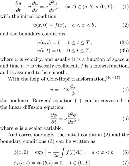
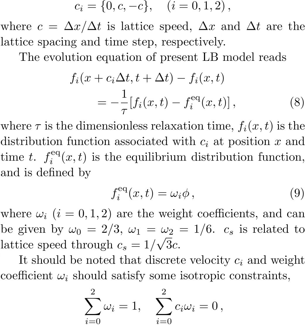
Now,we present an LB model for the linear diffusion equation(5).For simplicity but without losing generality,we only consider a simple D1Q3(three-discrete velocities in one dimension)lattice model,and three-discrete velocities in this lattice model can be given by

We now perform a detailed Chapman-Enskog analysis to derive converted linear diffusion from present LB model.In the Chapman-Enskog analysis,the distribution function,the time and space derivatives can be expended as

the linear diffusion equation(5)can be recovered exactly.

Finally,we would like to point out that,after computing?with present LB model,we also need to adopt Eq.(4)to calculate velocityu,and for this reason,some other special methods are also needed to compute?x?.Actually in previous studies,the term?x?is usually calculated by the traditional nonlocal FD schemes(e.g.,Ref.[46]).However in the framework of LB method,it can also be computed by the non-equilibrium part of the distribution function with a second-order convergence rate.[35?36,47]If we multiplyεon both sides of Eq.(22),and utilize the relation,one can derive an expression for computing

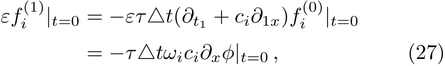
The initial value of equilibrium distribution functioncan be directly obtained through the initial condition(6),while the non-equilibrium partis unknown,and must be determined before performing any simulations.Based on Eq.(14),the initial value of nonequilibrium partcan be evaluated by

where Eqs.(9),(16),and(20)have been used.Actually,once the initial condition of?is given,one can determineand also the initial value of distribution functionfi.In addition,it should be noted that the termcan not be neglected in the initialization since it is not equal to zero,and also plays an important role in the computation of the term?x?and velocityu.

In summary,we developed a Cole-Hopf transformation based LB model for Burgers’equation and the algorithm can be found in the Appendix.

3 Numerical Results and Discussion

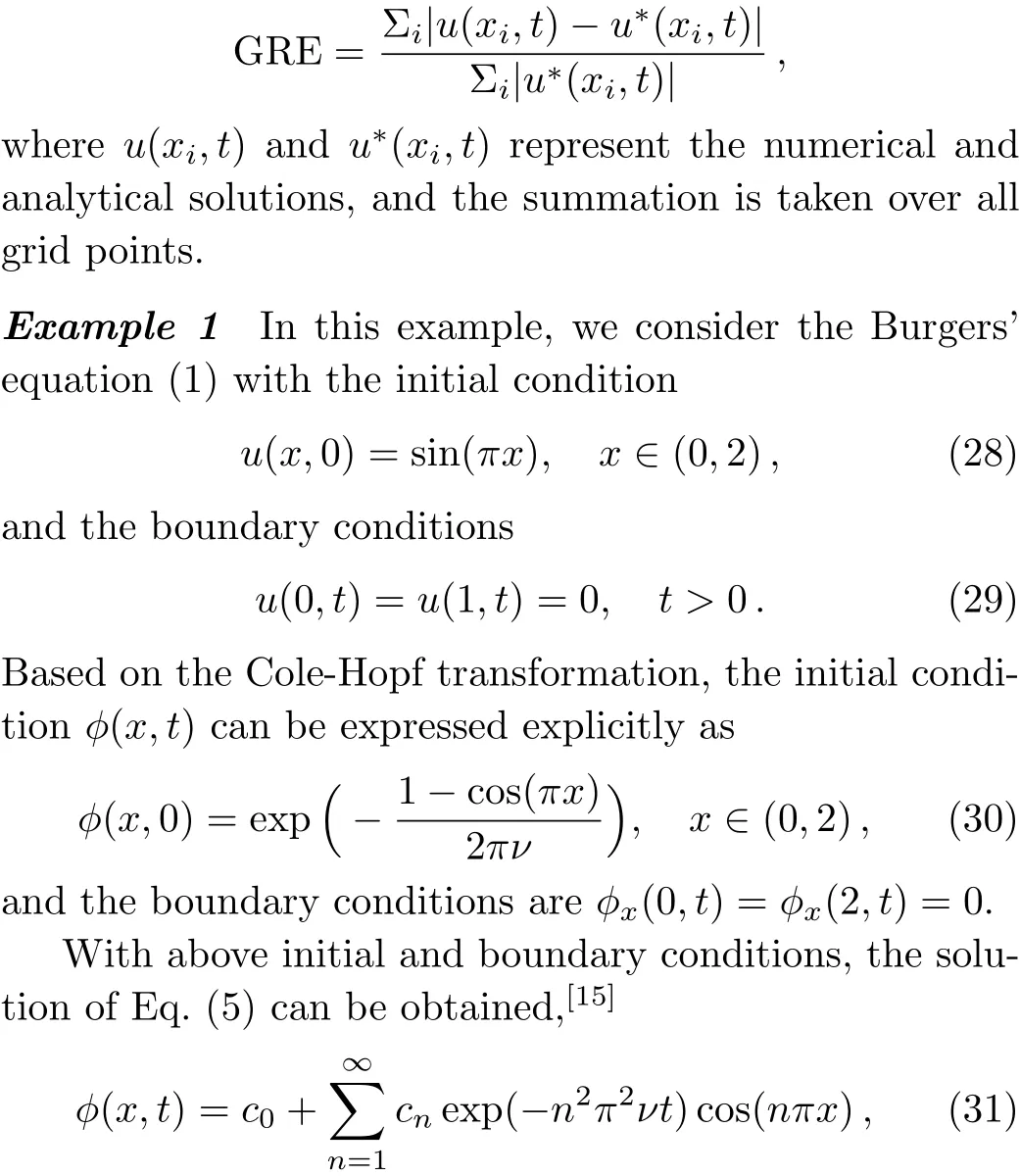
In this section,we conducted several numerical tests to validate present LB model,and to evaluate the accuracy of present model,the following global relative error(GRE)is adopted,

where the Fourier coefficients are given by

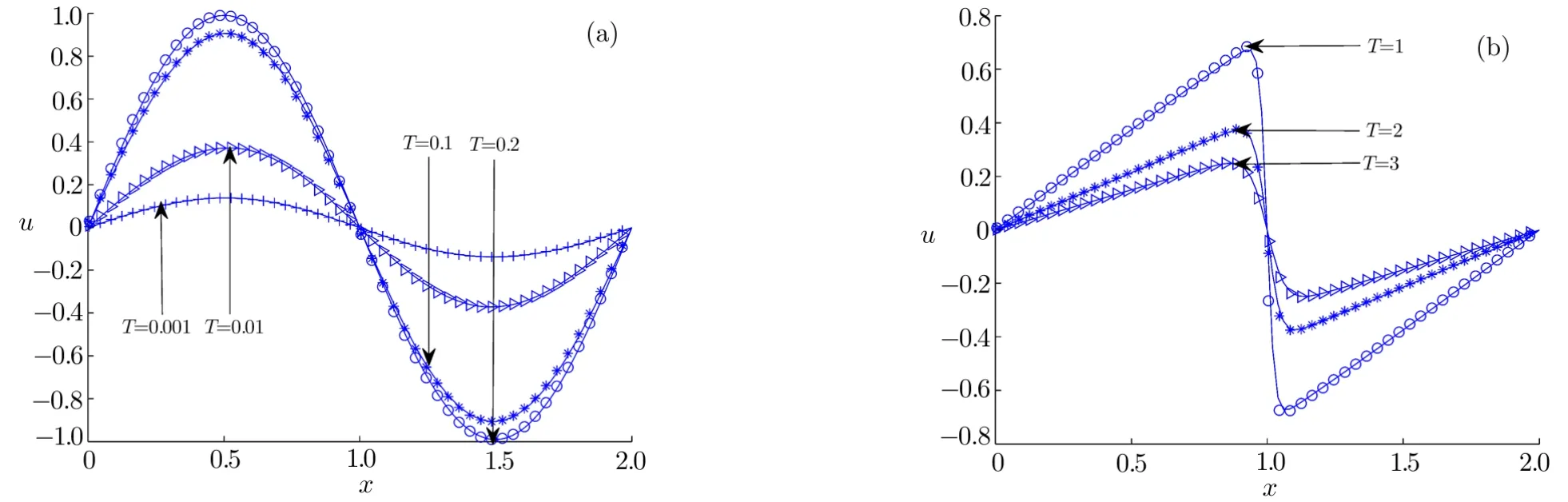
Fig.1 Numerical and analytical solutions at different time((a)ν=1.0,(b)ν=0.01;solid lines:analytical results,symbols:numerical results).

Table 1 A comparison between present LB model and some existing numerical methods(ν=1.0).

Table 2 A comparison between present LB model and some existing numerical methods(ν=0.01).

In our simulations,the computational domain is fixed to be[0,2],and the half bounce-back scheme is adopted for Neumann boundary conditions.[33,47?48]

We first carried out some simulations under different diffusion coefficients,and presented the result in Fig.1.As seen from this figure,the numerical results agree well with the corresponding analytical solutions.Then we also conducted a comparison between present LB model and some existing numerical methods,which are fully implicit finite-difference method(IFDM),[6]Douglas finite-difference method(DFDM),[8]B-spline finite element method(BFEM),[12]local discontinuous Galerkin method(LDG),[18]a mixed finite difference and boundary element method(BEM)[49]and Adomian’s decomposition method(ADM).[50]Based on the results listed in Tables 1 and 2,one can find that all numerical results are very close to the exact solutions,while the present model seems more accurate,especially for the case with a large diffusion coefficient.

Fig.2 Numerical and analytical solutions under different diffusion coefficients((a)ν=1.0,(b)ν=1.0×10?2,(c)ν=1.0×10?4,(d)ν=1.0×10?6;solid lines:analytical results,symbols:numerical results).

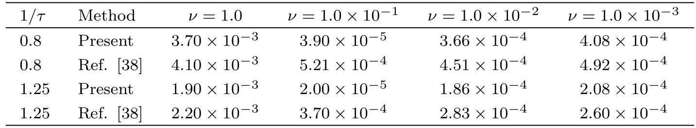
Table 3 GREs of two LB models for Example 2(?x=0.01,T=1.0).

Example 2To further examine the accuracy of our LB model,we also consider the example with the following initial condition

The exact solution to this problem can be expressed as[51]

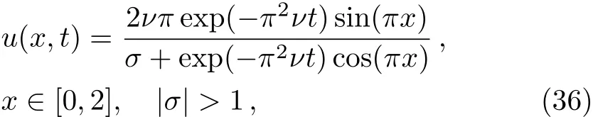
whereσis a parameter.

Similarly,with the help of Cole-Hopf transformation,we can also derive the exact solution to Eq.(1),

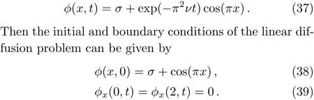
Fig.3 GREs of present LB model for Example 2(?x=1/10,1/20,1/25,1/40,1/50,1/80,1/100),the slope of the inserted line is 2.0,which indicates the present LB model has a second-order convergence rate.

In the following simulations,σis set to be 2,and the periodic boundary condition is adopted.We first performed some simulations,and presented the results in Fig.2 where ?x=0.01,T=1.0,andνis varied from 1.0 to 1.0×10?6.From this figure,it is clear that the numerical results are in agreement with the exact solutions.Then a comparison between present LB model and the traditional one[38]is also conducted,and the results are shown in Table 3 where?x=0.025,T=1.0,andνis varied from 1.0 to 1.0×10?3.From this table,one can find that the present LB model is more accurate than the traditional one in solving the Burgers’equation.Finally,to test the convergence rate of present LB model,we also carried out some simulations,and measured the GREs under different lattice sizes.Based on the results shown in Fig.3 whereν=1.0(1/τ=0.8)andν=0.01(1/τ=1.97),we can conclude that the present LB model has a second-order convergence rate in space.

4 Conclusions

In this paper,a new Cole-Hopf transformation based LB model is proposed for Burgers’equation.Compared to some available LB models,the present LB model is more accurate since the difficulty and error caused by nonlinear convection term can be avoided.On the other hand,the present LB model is also more efficient since a linear equilibrium distribution function is adopted.In addition,the numerical results also show that the present LB model has a second-order convergence rate in space.

In the next work,we would consider the Cole-Hopf transformation based LB models for two and threedimensional Burgers’equations.

Appdenix

In this appendix,we would present the algorithm of Cole-Hopf transformation based LB model.

#1.Computethrough Eq.(4).

#2.Computefi(x,0)at all points by Eq.(26),and the initial value of non-equilibrium partis calculated through Eq.(28).

#3.Conduct the collision process,and obtain the post-collision distribution functionat all points.

#4. Perform propagation at all points and derive

#5.Compute?xfrom Eq.(25),and calculatethrough Eq.(4).

#6.Implement steps#3–#5,and output the results at the speci fied timeT.

[1]L.Debnath,Sir James Lighthill and Modern Fluid Mechanics,Imperial College Press,London(2008).

[2]D.G.Crighton,Annu.Rev.Fluid Mech.11(2003)11.

[3]T.Nagatani,Rep.Prog.Phys.65(2002)1331.

[4]H.Bateman,Mon.Weather Rev.43(1915)163.

[5]J.M.Burgers,Adv.Appl.Mech.1(1947)171.

[6]BahadIr and A.Re fik,Int.J.Appl.Math.1(1999)897.

[7]W.Y.Liao,Appl.Math.Comput.206(2008)755.

[8]K.Pandey,L.Verma,and A.K.Verma,Appl.Math.Comput.215(2009)2206.

[9]Q.J.Li,Z.Zheng,and S.Wang,J.Appl.Math.14(2012)2607.

[10]S.Kutluay,A.R.Bahadir,and A.?zde?s,J.Comput.Appl.Math.103(1999)251.

[11]J.Caldwell,P.Wanless,and A.E.Cook,Appl.Math.Model.5(1981)189.

[12]S.Kutluay,A.Esen,and I.Dag,J.Comput.Appl.Math.167(2004)21.

[13]T.Ozis and A.Ozdes,J.Comput.Appl.Math.71(1996)163.

[14]W.Liao and J.Zhu,Int.J.Comput.Math.88(2011)2575.

[15]M.K.Kadalbajoo and A.Awasthi,Appl.Math.Comput.182(2006)1430.

[16]J.D.Cole,Q.Appl.Math.9(1951)225.

[17]E.Hopf,Commun.Pure Appl.Math.3(1950)201.

[18]R.P Zhang,X.Yu,and G.Zhao,Appl.Math.Comput.218(2012)8773.

[19]L.Shao,X.L.Feng,and Y.N.He,Math.Comput.Model.54(2011)2943.

[20]T.Krüger,H.Kusumaatmaja,A.Kuzmin,et al.,The Lattice Boltzmann Method—Princples and Practice,Springer,Switzerland(2017).

[21]S.Chen and G.Doolen,Annu.Rev.Fluid.Mech.30(1998)329.

[22]Z.L.Guo and C.Shu,Lattice Boltzmann Method and Its Applications in Engineering,World Scienti fic,Singapore(2013).

[23]S.Succi,The Lattice Boltzmann Equation for Fluid Dynamics and Beyond,Oxford University Press,Oxford(2001).

[24]Z.H.Chai,B.C.Shi,and L.Zheng,Chaos,Solitons&Fractals 36(2008)874.

[25]Z.H.Chai and B.C.Shi,Appl.Math.Model.32(2008)2050.

[26]G.W.Yan,J.Comput.Phys.161(2000)61.

[27]D.Wolf-Gladrow,J.Stat.Phys.79(1995)1023.

[28]C.Huber,B.Chopard,and M.Manga,J.Comput.Phys.229(2010)7956.

[29]B.C.Shi,B.Deng,R.Du,and X.W.Chen,Comput.Math.Appl.55(2008)1568.

[30]Z.H.Chai,B.C.Shi,and Z.L.Guo,J.Sci.Comput.69(2016)355.

[31]H.L.Wang,B.C.Shi,H.Liang,and Z.H.Chai,Appl.Math.Comput.309(2017)334.

[32]J.Huang and W.A.Yong,J.Comput.Phys.300(2015)70.

[33]H.Yoshida and M.Nagaoka,J.Comput.Phys.229(2010)7774.

[34]Q.H.Li,Z.H.Chai,and B.C.Shi,J.Sci.Comput.61(2014)308.

[35]Z.H.Chai and T.S.Zhao,Phys.Rev.E 90(2014)013305.

[36]Z.H.Chai and T.S.Zhao,Phys.Rev.E.87(6)(2013)063309.

[37]X.M.Yu and B.C.Shi,Chin.Phys.15(2006)1441.

[38]Y.Gao,L.H.Le,and B.C.Shi,Appl.Math.Comput.219(2013)7685.

[39]H.L.Lai and C.F.Ma,Physica A 395(2014)445.

[40]Q.H.Li,Z.H.Chai,and B.C.Shi,Appl.Math.Comput.250(2015)948-957.

[41]J.Y.Zhang and G.W.Yan,Physica A 387(2008)4771.

[42]Y.B.He and X.H.Tang,J.Stat.Mech.-Theory Exp.2016(2016)023208.

[43]Y.L.Duan and R.X.Liu,J.Comput.Appl.Math.206(2007)432.

[44]F.Liu and W.Shi,Commun.Nonlinear Sci.Numer.Simul.16(2011)150.

[45]A.C.Velivelli and K.M.Bryden,Physica A 362(2006)139.

[46]J.Wang,D.Wang,P.Lallemand,et al.,Comput.Math.Appl.65(2013)262.

[47]Z.H.Chai,C.S.Huang,B.C.Shi,and Z.L.Guo,Int.J.Heat Mass Transf.98(2016)687.

[48]I.Ginzburg,Adv.Water Resour.28(2005)1196.

[49]A.R.Bahadir and M.Saglam,Appl.Math.Comput.160(2005)663.

[50]S.Abbasbandy and M.T.Darvishi,Appl.Math.Comput.163(2005)1265.

[51]W.L.Wood,Int.J.Numer.Meth.Eng.22(2006)797.