
High Accuracy Split-Step Finite Difference Method for Schr¨odinger-KdV Equations?
2018-11-24 07:39:52FengLiao廖鋒andLuMingZhang張魯明
Feng Liao(廖鋒) and Lu-Ming Zhang(張魯明)
1School of Mathematics and Statistics,Changshu Institute of Technology,Changshu 215500,China
2College of Science,Nanjing University of Aeronautics and Astronautics,Nanjing 211106,China
AbstractIn this article,two split-step finite difference methods for Schr¨odinger-KdV equations are formulated and investigated.The main features of our methods are based on:(i)The applications of split-step technique for Schr¨odingerlike equation in time.(ii)The utilizations of high-order finite difference method for KdV-like equation in spatial discretization.(iii)Our methods are of spectral-like accuracy in space and can be realized by fast Fourier transform efficiently.Numerical experiments are conducted to illustrate the efficiency and accuracy of our numerical methods.
Key words:split-step method,Schr¨odinger-KdV equations,finite difference method,fast Fourier transform
1 Introduction
The nonlinear Schr¨odinger-KdV equations[1?2]
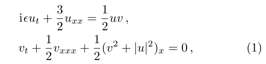
can be used to model the nonlinear dynamics behavior of one-dimensional Langmuir and ion-asoustic waves in a system of coordinates moving at the ion-acoustic speed.Here ? is a positive constant,u is complex function describing electric field of Langmuir oscillations while v is real function describing low-frequency density perturbation.
Many works have been concentrated on the numerical studies of this problem.Bai and Zhang[3]formulated a finite element method(FEM)to study Schr¨odinger-KdV equations. Later,Bai[4]developed a split-step quadratic B-spline finite element method(SSQBS-FEM)for Schr¨odinger-KdV equations.Appert and Vaclavik[5]solved the Schr¨odinger-KdV equations using a finite difference method(FDM).Golbabai a Safdari-Vaighani[6]employed a meshless technique based on radial basis function(RBF)collocation method.Zhang et al.did some works concerning Schr¨odinger-KdV equations using average vector field(AVF)method and multi-symplectic Fourier pseudospectral(MSFP)method.[7?8]Some other numerical methods for Schr¨odinger-KdV equations,such as variational iteration method,decomposition method and homotopy perturbation method,readers are reffered to Refs.[9–11]and reference therein.
The main purpose of this paper is to construct high accuracy split-step finite difference(SSFD)method for Schr¨odinger-KdV equations.Split-step(or time-splitting)method has evolved as a valuable technique for the numerical approximation of partial differential equations(PDE).Wang[12]presented a time-splitting finite difference(TSFD)method for various versions of nonlinear Schr¨odinger equation.To improve the accuracy of TSFD,Dehghan and Taleei[13]constructed a compact time-splitting finite difference scheme,which was proved to be unconditionally stable and preserve some invariant properties.Wang and Zhang[14]proposed an efficient split-step compact finite difference method for the cubicquintic complex Ginzburg-Landau equations both in one dimension and in multi-dimensions.However,all of these methods require to solve tridiagonal linear algebraic equations in implementation,and the computational cost will be increased along with the increment of the spatial accuracy.
Recently,Wang et al. constructed a time-splitting compact finite difference method for Gross-Pitaevskii equation,which is realized by discrete fast discrete Sine transform,and there is no need to solve linear algebraic equations.[15]Subsequently,Wang[16]considered sixthorder compact time-splitting finite difference method for nonlocal Gross-Pitaevskii equation,the method is of spectral-like accuracy in space,and conserves the total mass and energy of the system in the discretized level.It should be noted that the methods in Refs.[15–16]are notfit for solving the PDE with odd-order partial derivatives.In this paper,we formulate a high accuracy and fast solver for Schr¨odinger-KdV equations based on discrete Fourier transform,which is of sixth or eighth-order accuracy in space and can be realized by FFT efficiently.
The layout of the paper is as follows:In Sec.2,we formulate a sixth-order split-step finite difference(SSFD-6)method.Then we establish an eighth-order split-stepfinite difference(SSFD-8)method in Sec.3.Numerical investigations of our numerical methods are conducted in Sec.4,and some conclusions are drawn in Sec.5.
2 Sixth-Order Split-Step Finite Difference Method
In this paper,we consider the general forms of Schr¨odinger-KdV equations
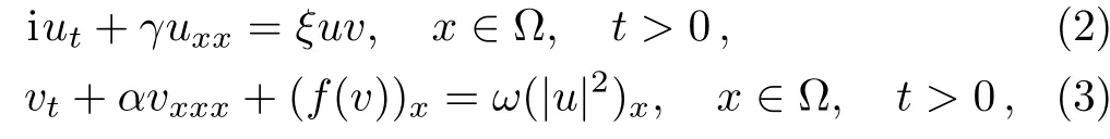
with the initial value and periodic-boundary conditions of
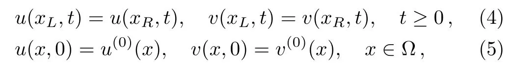
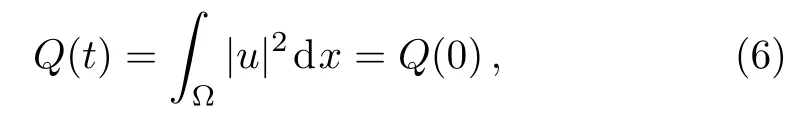
where ? =[xL,xR],γ,ξ,α,ω are known constants,u(0)(x)and v(0)(x)are periodic functions with the period xR?xL.It is easy to verify that problem(2)–(5)preserves the total mass
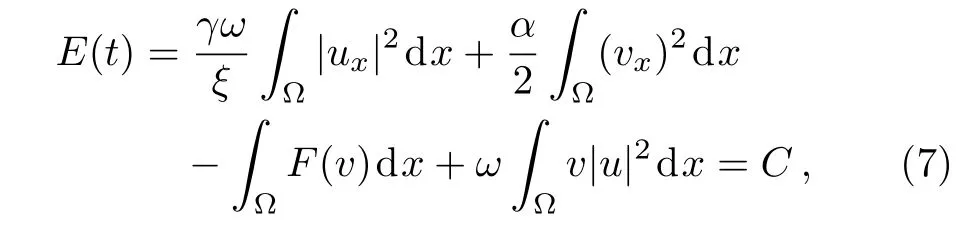
and the total energy
2.1 Sixth-Order Difference Approximation Formula
Choose a mesh size h:=(xR?xL)/J with J an even positive integer,time step τ,and denote grid points with coordinates(xj,tn):=(xL+jh,nτ)for j=0,1,...,J?1 and n≥0.Define
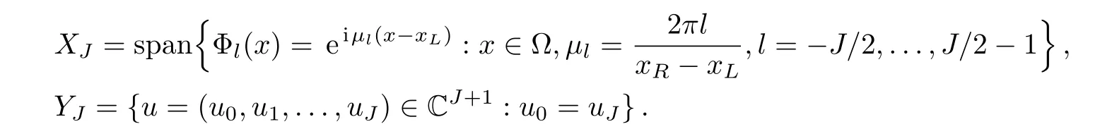
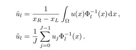
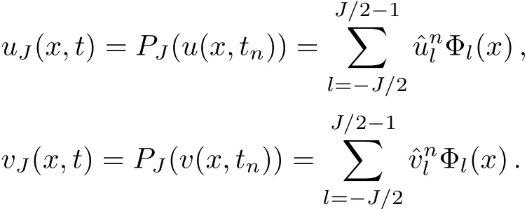
For any general periodic function u(x)on ? and a vector u ∈ YJ,let PJ:L2(?)→ XJbe the standard L2-projection operator onto XJ,IJ:C(?) → XJand IJ:YJ→XJbe the trigonometric operator,i.e.
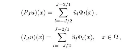
with
Obviously,PJand IJare identical operators over XJ.
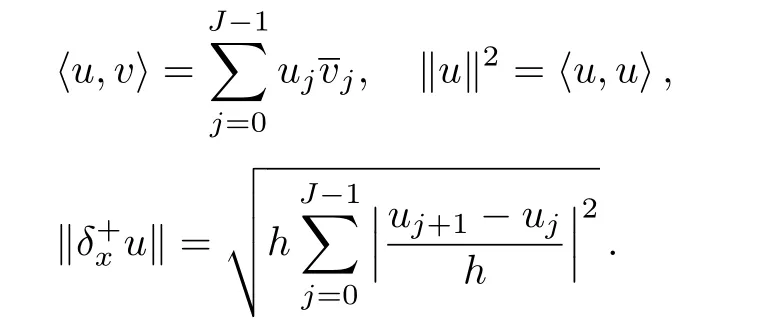
For any u,v∈YJ,the inner product and norm are defined as follows:
Suppose that g(x)is an xR?xLperiodic function,then for the approximation of the first-order derivative gx(x),we have the following formula,i.e.
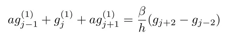
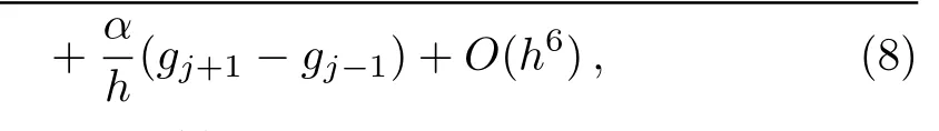
where gj=g(xj),=gx(xj)and a,α,β are undetermined parameters,which depend on the accuracy-order constraints.Base on Taylor’s expansion,we have

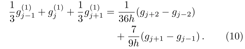
The linear equations(9)is unique solvable,i.e.a=1/3,α=7/9,β=1/36.Then we obtain the sixth-order difference approximation for the first-order partial derivative
Next,we approximate the third-order derivative fxxx(x)via the following formula,i.e.
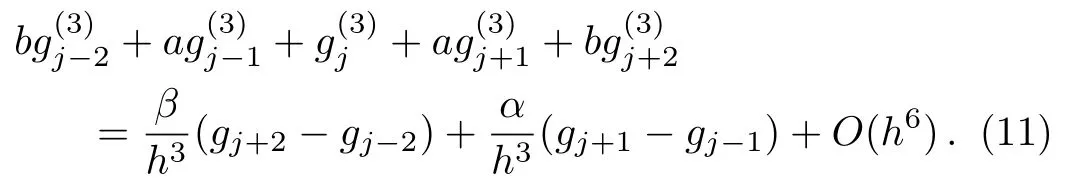
It follows from Taylor’s expansion,we obtain
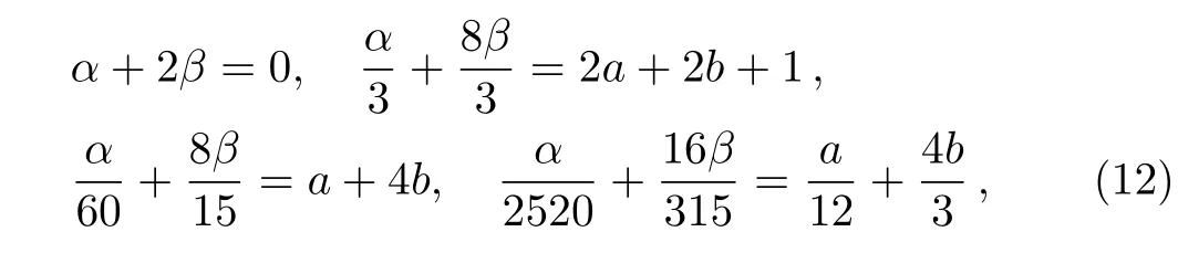
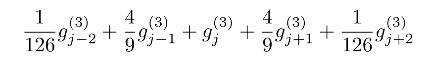
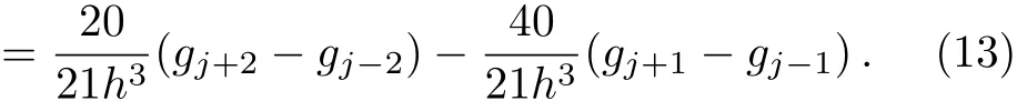
which is unique solvable,i.e. a=4/9,b=1/126,α= ?40/21,β=20/21.Thus,the sixth-order difference approximation for the third-order partial derivative is given as follows
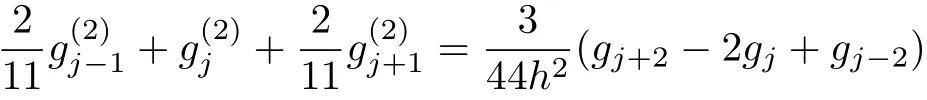
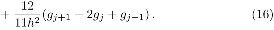
Finally,we approximate the second-order derivative fxx(x)as follows
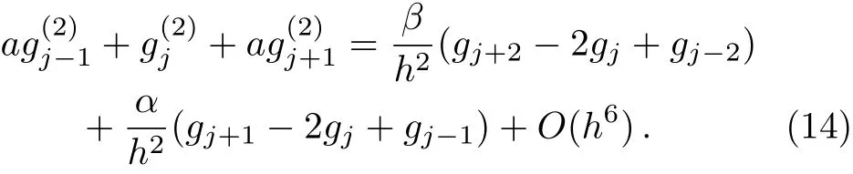
From Taylor’s expansion,we have

which is unique solvable and a=2/11,α=12/11,β=3/44.Then the sixth-order difference approximation for the second-order partial derivative is given as follows
2.2 Split-Step Finite Difference Method
The discrete Fourier transform for{gj}and its inverse are provided as follows,i.e.
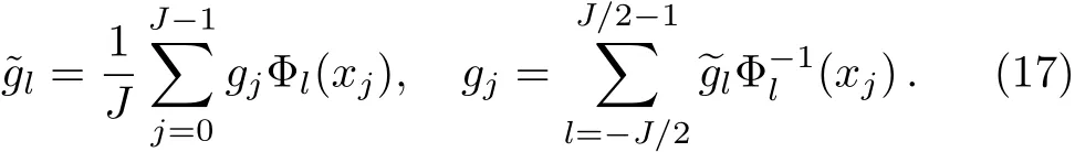
Similarly,wa can define discrete Fourier transform for,,andand their inverse.
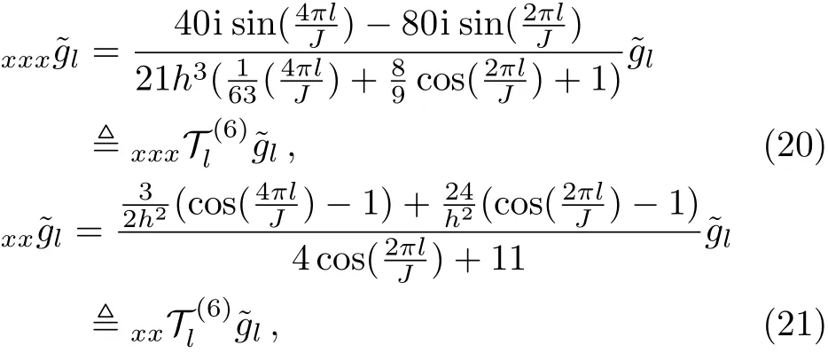
From Eqs.(10)and(17),we have
which gives
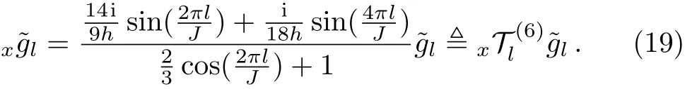
Similarly,from Eqs.(13),(16),and(17),we obtain
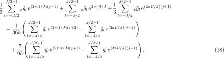
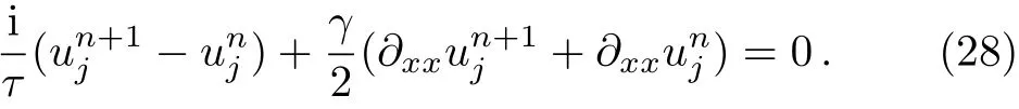
In the rest of this section,we formulate a splitstep finite difference(SSFD)method for problem(2)–(5).Firstly,we discrete KdV-like equation(3)in temporal direction as follows
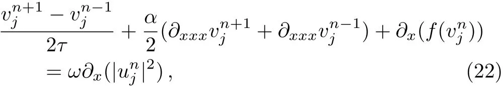
for j=0,1,...,J?1.Acting the discrete Fourier transform on Eq.(22)and considering the orthogonality of the Fourier basis functions,we obtain

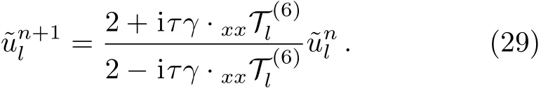
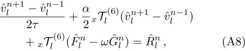
for l=?J/2,?J/2+1,...,J/2?1,where,,andrepresent the discrete Fourier transform of,,and,respectively.From Eqs.(19),(20)and(23),we obtain
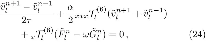
for n≥ 1 and l= ?J/2,?J/2+1,...,J/2?1,whereandexpress the discrete Fourier transform ofand,respectively.
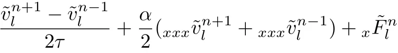
Secondly,we utilize split-step method to discrete Schr¨odinger-like equation(2)in time,we obtain
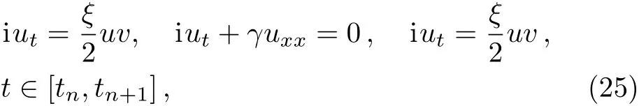
Directly from the nonlinear subproblem in Eq.(25),we have
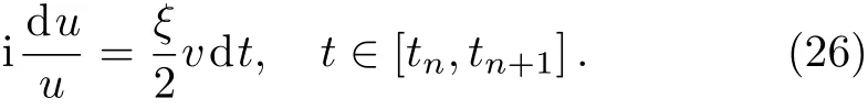
Integrating Eq.(26)from tnto tn+1,and then approximating the integral on[tn,tn+1]via trapezoidal rule,we obtain

For the linear subproblem in Eq.(25),we discretize it in time as follows
Followed by discrete Fourier transform and Eq.(21),we have
From Eqs.(27)and(29),the sequential subproblems(25)can be solved as follows:
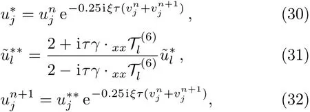
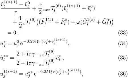
From above discussion,Eqs.(24)and(30)–(32)comprise the details of sixth-order split-step finite difference(SSFD-6)method. However,SSFD-6 is a three-level scheme,which requires a two-level scheme to calculate u1and v1.In this article,we compute u1and v1via the following two-level nonlinear implicit scheme,i.e.
Above all,the details of SSFD-6 are provided as follows:
DO
END WHILE
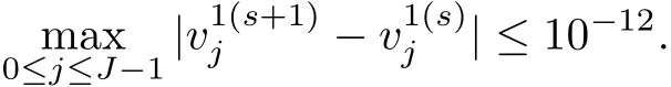
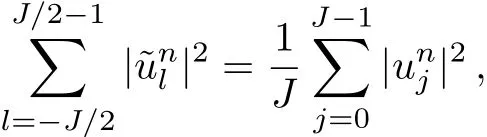
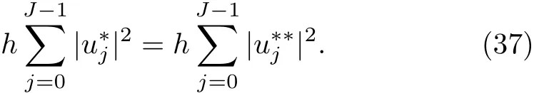
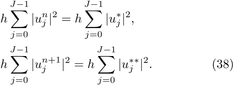
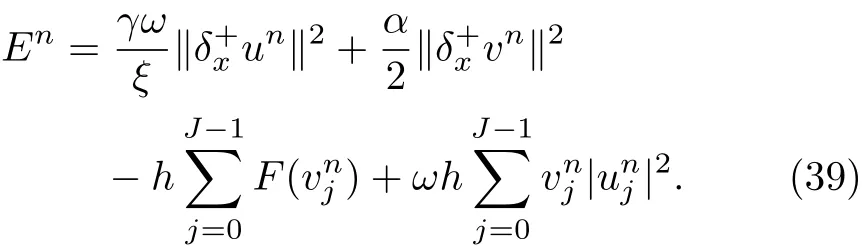
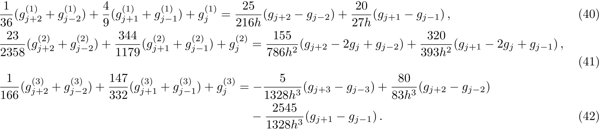
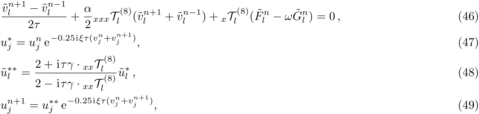
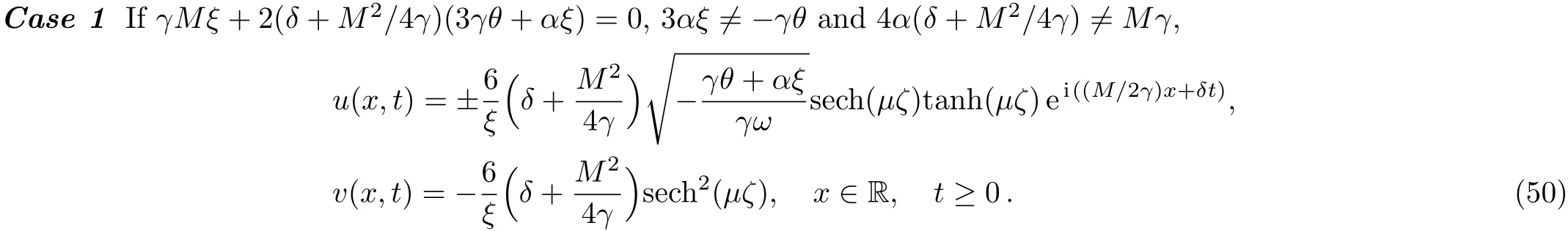
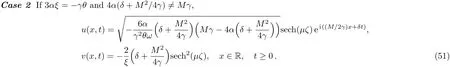
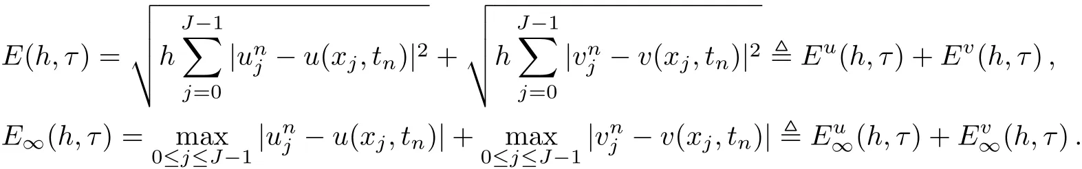
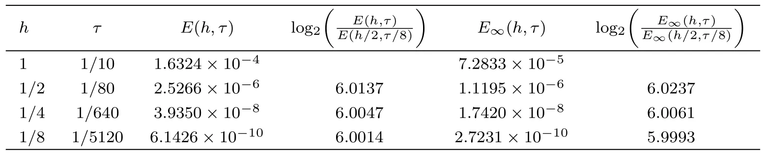
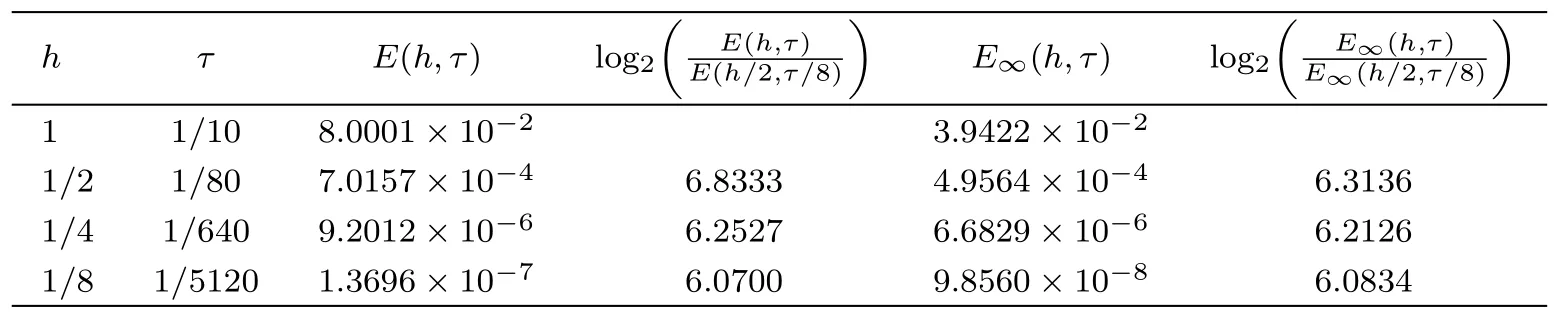
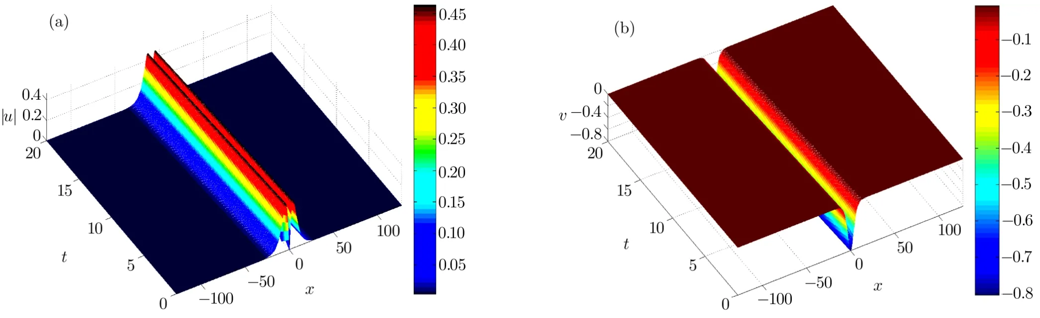
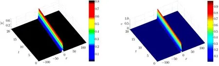
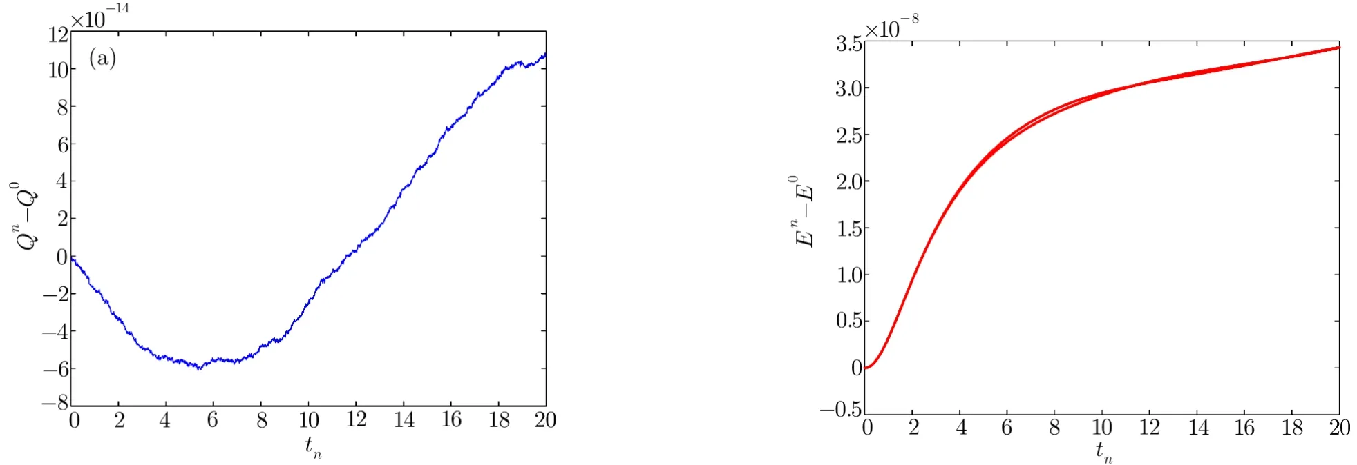
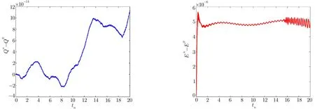
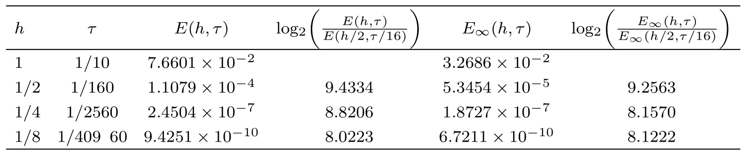
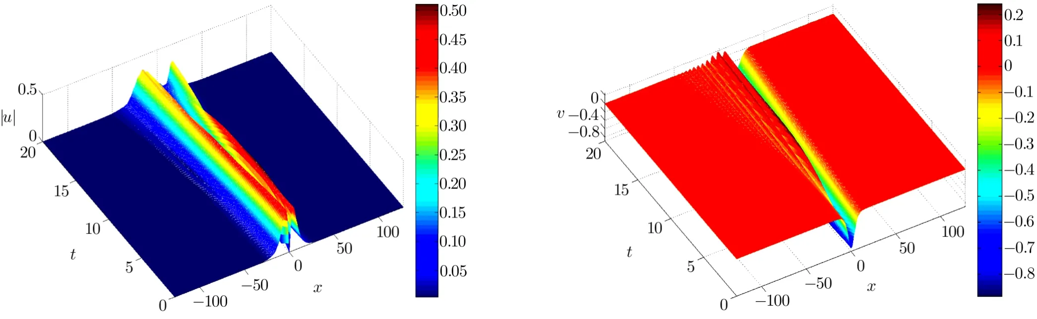
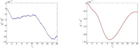
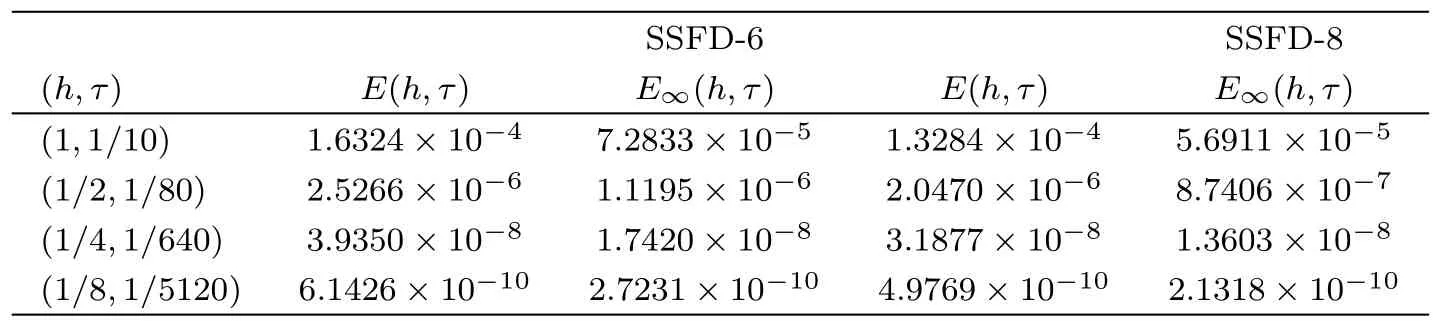
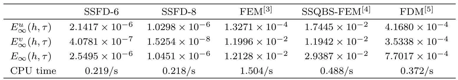
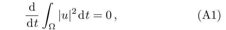
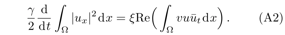
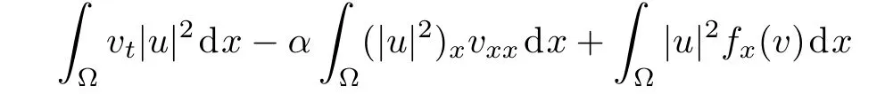
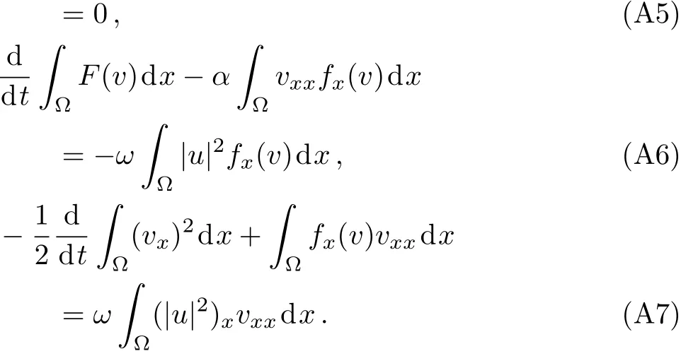
WHILE n DO END WHILE Theorem 1 The discretizations Eqs.(30)–(32)for Sch¨odinger-like equation posses the following property: where Qn= ∥un∥2. Proof Noticing the Parserval’s identity thus from Eq.(31),we have Directly from Eqs.(30)and(32),we have From Eqs.(37)and(38),we can see that the conclusion of this theorem holds. ? Remark 1 Theorem 1 implies that SSFD-6 method preserves the total mass in discrete level.We do not expect that SSFD-6 conserves the total energy,but the energy can be discretized as Theorem 1 also demonstrates that the complex component unis convergent in the sense of L2-norm.Similar to the methods which have been done in Ref.[17],we can obtain the L2-error estimates of un,i.e. where C0is a constant independent of h,τ.For simplicity of this paper,we omit the proof details.Next,we will prove the convergence of vnvia mathematical induction argument method. Theorem 2 Let un,vn∈XJbe the numerical approximations of SSFD-6.If u(x,t),v(x,t),and f(·)are sufficiently smooth,there exist two constants h0>0 and C independent of τ(or n)and h,such for any h ≤ h0and τ=o(h), Proof See Appendix B. ? To construct eighth-order split-step finite difference(SSFD-8)method for Schr¨odinger-KdV equations,we provide the eighth-order finite difference formulas for the first,second and third-order derivatives as follows: This together with Eq.(17),we obtain the relationship betweenx?gl,xx?gl,xxx?gl,and?glas follows Similar to the analysis in Sec.2,the details of SSFD-8 are provided as follows for n ≥ 1,and u1,v1can be calculated iteratively as we have done in Eqs.(33)–(36). Comparing with SSFD-6,we can see that the computational complexity of SSFD-8 is identical to SSFD-6,but SSFD-8 is more accurate than SSFD-6 in spatial direction.Thus the computational complexity of our methods will not increase along with the increment of spacial accuracy.Based on this,we can design more higher accurate SSFD method,which can achieve spectral-like accuracy in space when more higher-order finite difference method is investigated. In this section,we will provide some numerical examples to test the performance of SSFD method for Schr¨odinger-KdV equations.Based on the works of Refs.[2,18],we provide two kinds of solitary-wave solutions for problem(2)–(3)with f(v)=θv2. Example 1 Let γ=3/2,ξ=1/2,α =1/2,θ=1/2,ω =?1/2,and M=?9/20,δ=27/800. Example 2 Let γ=1,ξ=?1,α =1/3,θ=1,ω =?1/2,and M=1,δ=1/4. We calculate the L2and L∞norm errors using the formulas Table 1 The errors and convergence ratio of SSFD-6 for Example 1 at t=1 with ?=[?128,128]. Table 2 The errors and convergence ratio of SSFD-6 for Example 2 at t=1 with ?=[?128,128]. Fig.1 Numerical solutions of Example 1 for t ∈ [0,20]with ? =[?128,128]. The errors and convergence ratio of SSFD-6 are examined in Tables 1–2,which demonstrate that SSFD-6 has sixthorder accuracy in space.Figures 1 and 2 simulate the numerical solutions of SSFD-6 for Example 1 and Example 2,respectively,with h=1/2 and τ=1/80. Fig.2 Numerical solutions of Example 2 for t∈ [0,20]with ? =[?128,128]. Fig.3 The discretization errors of the conservative quantities for Example 1 with h=1/2,τ=1/80 and ? =[?128,128]. Fig.4 The discretization errors of the conservative quantities for Example 2 with h=1/2,τ=1/80 and ? =[?128,128]. From Table 3,we can see that SSFD-8 is of eighth-order accuracy in space.We have compared the accuracy of SSFD-6 and SSFD-8 in Table 4,which indicates that SSFD-8 is more accurate than SSFD-6. Table 3 The errors and convergence ratio of SSFD-8 for Example 2 at t=1 with? =[?128,128]. Fig.5 Numerical solutions of general nonlinearity for t∈ [0,20]with h=1/2,τ=1/80 and ? =[?128,128]. Fig.6 The discretization errors of the conservative quantities for general nonlinearity with h=1/2,τ=1/80 and? =[?128,128]. Table 4 Comparison of L2and L∞error norms for numerical solutions of Example 1 at t=1 with ? =[?128,128]. To validate the conservation properties,we have computed the total mass and energy of Example 1 and Example 2,the discretization errors of the conservative quantities are plotted in Fig.3 and Fig.4,which demonstrate that SSFD-6 preserves the total mass and energy very well.A comparative study has been conducted with some existing methods and the results are reported in Table 5.We choose quadratic spline functions as basis functions of FEM[3]and SSQBSFEM[4]for spacial discretization.From Table 5,we can see that SSFD-6 and SSFD-8 are more efficient and accurate than other three methods.As can be seen from Table 5 that SSFD-8 is more accurate than SSFD-6,but the complexity of SSFD-8 is identical to SSFD-6.It should be pointed that the standard fourth order Runge-Kutta method is used to solve the continuous time system of FEM,[3]hence FEM[3]is expected to spent more CPU time than SSQBS-FEM.[4]Since the coefficient matrix of FDM[5]is time-varying when we evaluate the complex component un,hence FDM[5]requires more computational time than SSFD-6 and SSFD-8. Table 5 Comparison of L∞error norms for numerical solutions of Example 1 at t=0.1 with h=1,τ=0.001 and ? =[?64,64]. To examine SSFD-6 still works for the general nonlinearity,we take in the Schr¨odinger-KdV Eqs.(2)–(3)with f(v)=sin(v).Choosing the parameters γ,ξ,α,ω and the initial data same as Example 1,the corresponding numerical results are shown in Fig.5 and the discretization errors of the conservative quantities are plotted in Fig.6. In this paper,two split-step finite difference methods are presented for solving Schr¨odinger-KdV numerically.The merit of our methods are of spectral-like accuracy in space and can be realized by fast Fourier transform.The computational complexity of our methods will not increase along with the increment of spacial accuracy.Numerical results demonstrate the precision and conservation properties of our methods. Appendix A ProofMaking the complex conjugate inner product of Eq.(2)with u,then taking the imaginary part,we get which implies that Eq.(6)holds. Computing the the complex conjugate inner product of Eq.(2)with ut,then taking the real part,we have Followed by then we obtain Making the inner product of Eq.(3)with|u|2,f(v)and vxx,respectively,we obtain It follows from(A5)–(A7)that(7)is satisfied. ? Appendix B Denote the trigonometric interpolations of the numerical solutions as where un,vn∈ YJ.Define the“error”functions Denote the L2-projected solutions as Acting L2-projected operator on Eq.(3),using Taylor’s expansion and considering the orthogonality of the basis functions,we have Noticing With the help of mathematical induction argument,we assume that This together with the inverse inequality,triangle inequality and Sobolev inequality,we have Considering the conditions of Theorem 2 and(A13),we obtain It follows from Parserval’s identity and(A10)–(A13),we have Directly from(A15)and induction argument(A12),we have where C is a constant independent of τ and h.This completes the proof. ?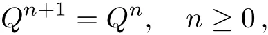


3 Eighth-Order Split-Step Finite Difference Method
4 Numerical Results
5 Conclusion


 Communications in Theoretical Physics2018年10期
- Communications in Theoretical Physics的其它文章
- P-V Criticality of Born-Infeld AdS Black Holes Surrounded by Quintessence?
- Baryogenesis in f(R,T)Gravity?
- Prospect for Cosmological Parameter Estimation Using Future Hubble Parameter Measurements?
- Topological Dark Matter from the Theory of Composite Electroweak Symmetry Breaking?
- Pair Production in Chromoelectric Field with Back Reaction?
- Impact of Internal Heat Source on Mixed Convective Transverse Transport of Viscoplastic Material under Viscosity Variation