
Theoretical framework for geoacoustic inversion by adjoint method?
2019-11-06 00:44:44YangWang汪洋andXiaoFengZhao趙小峰
Chinese Physics B 2019年10期
關(guān)鍵詞:汪洋
Yang Wang(汪洋) and Xiao-Feng Zhao(趙小峰)
1School of Marine Science and Technology,Northwestern Polytechnical University,Xi’an 710072,China
2Key Laboratory of Marine Intelligent Equipment and System of Ministry of Education,Shanghai Jiao Tong University,Shanghai 200240,China
3College of Meteorology and Oceanography,National University of Defense Technology,Nanjing 211101,China
Keywords:geoacoustic inversion,adjoint method,parabolic equation,non-local boundary condition
1.Introduction
Sound wave is the only information carrier that can travel long distances in the ocean.The exploration and development of marine resources,underwater target detection and identification,and environmental monitoring are all dependent on underwater acoustic detection technology.[1–3]Accurate acquisition of geoacoustic parameters is a prerequisite for the effective implementation of this technology.Due to the complexity of the marine environment,it is difficult for traditional in situ methods to obtain large-scale geoacoustic parameters in real time.With the advancement of sonar technology and inverse problem theory,the use of acoustic signals to invert the parameters of underwater acoustic environments has received more and more attention.[4–6]
Most previous geoacoustic studies have focused on using matched-field processing methods in combination with heuristic searching methods,such as genetic algorithm,[7]simulated annealing,[8]and sequential Monte Carlo sampling,[9]which always need huge computing resources because of too many forward propagation model runs. The adjoint method coming from optimal control theory is known to give accurate and efficient data assimilation processes in oceanography and meteorology.[10,11]However,it has rarely been applied in underwater acoustics for inversion purposes.[12]
For underwater acoustics modelling,a downgoing radiation condition must be imposed on the transmitted component of the field since the seabed is penetrable to sound waves,especially at low frequencies.Although many acoustic propagation tools are now available,the parabolic equation(PE)model has the advantages of dealing with the range-dependent environments efficiently and obtaining the full wave solution of the sound field.In the PE models,a downgoing radiation condition can be done by appending an absorbing layer[13]or alternatively by applying a non-local boundary condition(NLBC).[14]The latter is more attractive for limiting the computations in the interested region and time saving.
The remainder of this paper is organized as follows:The forward propagation model,i.e.,a non-local boundary condition for the finite-difference PE solver,is briefly introduced in Section 2.Section 3 presents the detailed theoretical derivations of the geoacoustic inversion by variational approach,including the tangent linear model,adjoint operator,and the gradients of the cost function with respect to the control variables.The iteration process is given in Section 4.
2.Forward propagation model
With the far-field assumption and paraxial approximation,the standard PE can be written as[13]
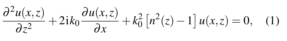
where x is the range and z is the depth,u(x,z)is a slowly varying function related to the complex acoustic pressure fieldis the zeroth order Hankel function,k0=2π f/c0is a reference wave number,f is the source frequency,and c0is a reference sound speed.Term n(z)=c0/c(z)is the refractive index,and c(z)is the sound speed of the water column.
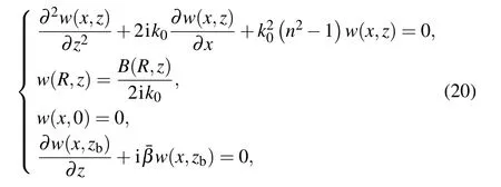
To obtain a well-posed initial boundary value problem of Eq.(1),an initial field u(0,z)=S(zs,z)(S is an initial field function and zsis the source depth)and a perfectly reflecting interface condition u(x,0)=0 at the sea surface are used.The NLBC formulation at the water–sediment interface z=zb,proposed by Yevick and Thomson,[14]is used as the lower boundary. Dividing the propagation range 0 →x+?x into L+1 intervals of width ?x,and denoting uj=u(x ?j?x,zb)and x=(L+1)?x,the NLBC can be expressed as

where ρwand ρbindicate the density of water column and sediment,respectively.Nb=(c0/cb)·[1+iαb],where cband αbare the sound speed and the absorption loss of the sediment,respectively.ν2=4i/(k0?x)and gjare the coefficients derived from the Taylor expansion of the vertical wave number operator,Γ0in powers of the translation operator=exp(??x?x).Thus,the standard PE model with initial and boundary conditions can be summarized as

Equation(5)can be solved by the implicit Crank–Nicolson finite difference method.Once the field u(x,z)is obtained,the transmission loss T(x,z)in unit dB is then given by

3.Framework of the inverse problem
3.1.Cost function
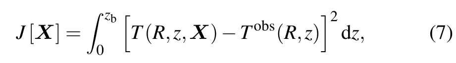
Note the computation domain be[0,R]×[0,zb],and a vertical line array locating at a given range R receive the field measurementsThen,the control procedure consists of finding the optimal control variables which minimize a cost functionas
3.2.Tangent linear model
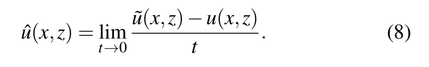
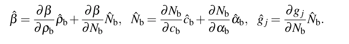
Set perturbations to c(z),cb,ρb,and αbasandthen the corresponding perturbations of β and gjcan be described asandrespectively.Noteis the Gateaux differential of u(x,z)
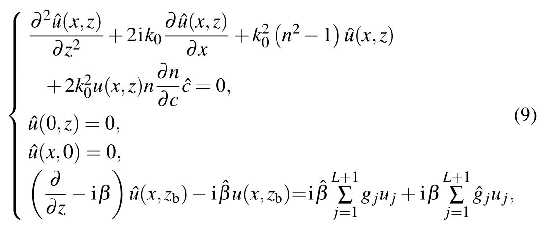
where
3.3.Adjoint model

in which

Combining the above four equations and considering the lower boundary layer of the tangent linear model,

where

Now return to the cost function,the Gateaux differential ofwith respect toat pointis

On the other hand,according to the definition we can get
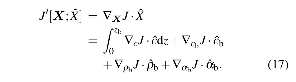
According to Eq.(16)and Eq.(17),

where
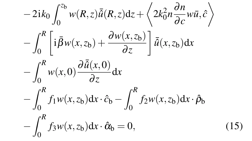
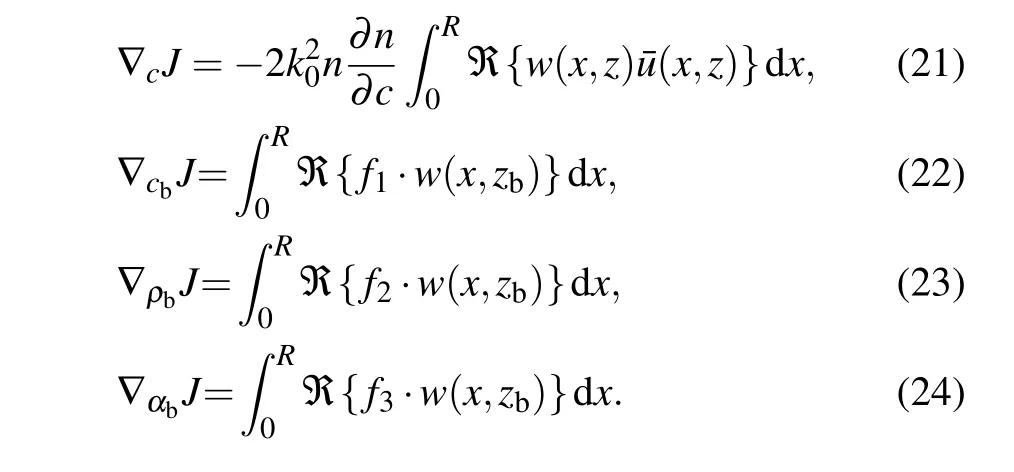
Combining Eq.(15)with Eq.(18),

and the corresponding gradients of the cost function respective to the control variables are
4.Iteration process
With these gradients,optimization could be generally accomplished through using the iterative gradient-based methods,
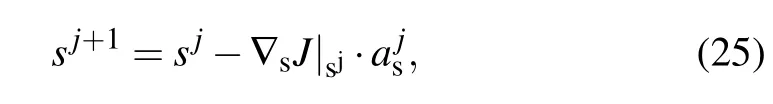
The flowchart of the whole iteration process is shown in Fig.1.Starting with a first guess of the control vector,the forward model runs to give the corresponding complex field u(x,z)and the replica transmission loss T(R,z).Then,the resulting mismatches between model results and observations are used to initiate the adjoint model which can also be solved by the implicit Crank–Nicolson finite difference method.With the adjoint information thus obtained,the gradients of the cost function are determined and the current control vectoris updated accordingly to start the next iteration until the criteria for the solutions are met.

Fig.1.The flowchart of the iteration process for geoacoustic inversion by adjoint NLBCPE method,where“0 →R”means integrating the forward model along the range 0 to R,and“R →0”means integrating the adjoint model in the reverse direction.
5.Discussion and conclusion
The analytical theory framework for geoacoustic inversion by the adjoint PE method is introduced above.It should be noted that parameter estimation problems have demonstrated to be ill-posed,especially when the problems are severely nonlinear and the observed data are contaminated by noise.[15]These problems usually have multiple local optimal solutions.To deal with the ill-posedness of the inversion,an efficient method is to carry out regularization that can make the cost function be convex. Detailed regularization techniques for inverse problem can refer to Ref.[16].
On the other hand,the theoretical derivations are based on small perturbation approach. Therefore,the adjoint process is a local optimization method and the inversion accuracy is dependent on the initial guess,[17]especially for severely nonlinear inverse problems.If the initial guess is deviated far from the true solution,the iterations will be always trapped to a local optimal solution.In practical operations,a good initial guess can be obtained from historical observations and/or empirical values.
Geoacoustic parameters are very important for underwater acoustic detection.How to acquire these parameters accurately from the perspective of adjoint PE method needs systematical research.This paper only gives the basic theoretical framework,and future work will be focused on discussing the uniqueness and stability of the solution,as well as collecting the experimental data to validate this theoretical method.
猜你喜歡
Chinese Physics B(2021年3期)2021-03-19 03:24:50
今日農(nóng)業(yè)(2020年21期)2020-12-19 13:52:28
收藏與投資(2020年12期)2020-04-18 07:31:06
當代陜西(2018年6期)2018-05-22 03:03:21
中國三峽(2016年9期)2017-01-15 13:59:40
中國老區(qū)建設(shè)(2016年4期)2017-01-15 13:53:35
中國火炬(2015年7期)2015-07-31 17:39:57
創(chuàng)業(yè)家(2015年1期)2015-02-27 07:52:18
中國火炬(2014年1期)2014-07-24 14:16:47
中國火炬(2013年11期)2013-07-25 09:50:21

- Chinese Physics B的其它文章
- Theoretical analyses of stock correlations affected by subprime crisis and total assets:Network properties and corresponding physical mechanisms?
- Influence of matrigel on the shape and dynamics of cancer cells
- Benefit community promotes evolution of cooperation in prisoners’dilemma game?
- Theory and method of dual-energy x-ray grating phase-contrast imaging?
- Quantitative heterogeneity and subgroup classification based on motility of breast cancer cells?
- Designing of spin filter devices based on zigzag zinc oxide nanoribbon modified by edge defect?