Existence and Multiplicity of Periodic solutions for the Non-autonomous Second-order Hamiltonian Systems

CHEN Yu-song, CHANG He-jie

(1.Department of Basic Education, Shangqiu Institute of Technology, Henan, 476000, P.R. China;2.Department of Basic Education, Luohe Vocational Technology College, Henan, 462000, P.R. China)

Abstract: In this paper, we study the existence and multiplicity of periodic solutions of the non-autonomous second-order Hamiltonian systemswhere T > 0. Under suitable assumptions on F, some new existence and multiplicity theorems are obtained by using the least action principle and minimax methods in critical point theory.

Key words: Periodic solution; Second-order Hamiltonian system; Saddle Point Theorem;Sobolev’s inequality; Wirtinger’s inequality

§1. Introduction and Main Results

Consider the non-autonomous second-order Hamiltonian systems

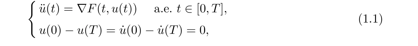
where T >0, F :[0,T]×RN→R satisfy the following assumption:

(A) F(t,x) is measurable in t for every x ∈RNand continuously differentiable in x for a.e.t ∈[0,T], and there exist α ∈C(R+,R+), b ∈L1(0,T;R+) such that

for all x ∈RNand a.e. t ∈[0,T].

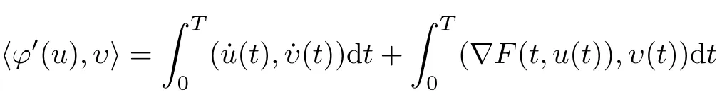
The corresponding function ? on H1Tgiven by

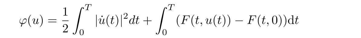
is continuously differentiable and weakly lower semi-continuous on H1T, where

is a Hilbert space with the norm defined by

As is well known, a Hamiltonian system is a system of differential equations which can model the motion of a mechanical system. An important and interesting question is under what conditions the Hamiltonian system can support periodic solutions. During the past few years,many existence results are obtained for problem(1.1)by the least action principle and the minimax methods (see[1-2, 4-6, 8-13, 14-25]). Using the variational methods, many existence results are obtained under different conditions, such as the coercive condition (see [1,5]), the periodicity condition (see [2, 5]), the convexity condition (see [4, 5, 7, 9]), the subconvex condition (see [15-16, 19]) and the subaddieive condition (see [7, 16]).

Especially,when the gradient ?F(t,x)is bounded,that is,there exists g(t)∈L1([0,T],R+)such that

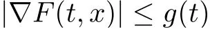
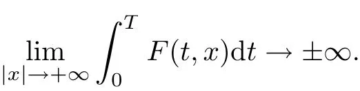
for all x ∈RNand a.e. t ∈[0,T], Mawhin and Willem [5]proved the existence of solutions for problem (1.1) under the condition

When the gradient ?F(t,x)is sublinearly bounded,that is,there exist f, g ∈L1(0,T;R+)and α ∈[0,1) such that

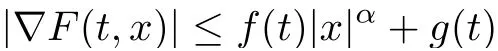
for all x ∈RNand a.e. t ∈[0,T], Tang [8]also proved the existence of solutions for problem(1.1) under the condition

which generalizes Mawhin-Willem’s results.

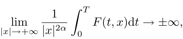
Afterwards, Y.W Ye and C.L Tang [20]study the existence and multiplicity of periodic solutions by the following conditions:

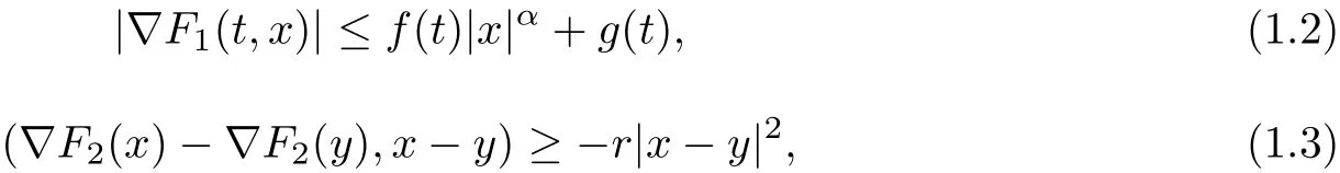
where r <4π2/T2, f,g ∈L1(0,T;R+), α ∈[0,1) and F =F1+F2.

Inspired and motivated by the results due to Y.W Ye[20], R.G Yang[16], Nurbek Aizmahin and T.Q An [19], X.H. Tang and Q. Meng [22], X.Y. Zhang and Y.G. Zhou [15], Z. Wang and J. Zhang [13], J. Pipan, M. Schechter [23], we will focus on some new results for problem (1.1)under some more general conditions then (1.2) and (1.3).

In the following,we always suppose that F(t,x)=F1(t,x)+F2(t,x)satisfies the assumption(A), we will use the following conditions for F1, F2.

(F1) There exists constants C0> 0, K1> 0, K2> 0, α ∈[0,1) and a nonnegative function h ∈C([0,∞),[0,∞)) with the properties:

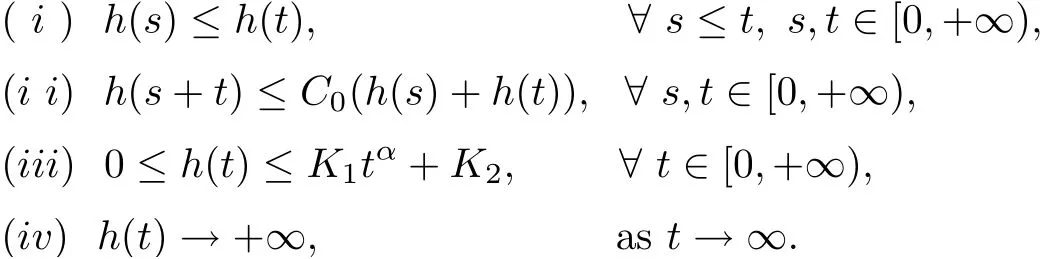
Moreover, there exist f ∈L1(0,T;R+) and g ∈L1(0,T;R+) such that

for all x ∈RNand a.e. t ∈[0,T].

(F2) there exists r ∈L1(0,T;R+) withr(t)dtsuch that

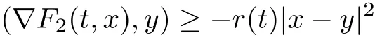
for all x,y ∈RNand a.e. t ∈[0,T].

We know the condition (F1), (F2) are more weakly than the condition (1.2) and (1.3). In fact, the condition (1.2) is special cases of the condition (F1) with control function h(x)=xα,α ∈[0,1), t ∈[0,∞). Then the existence of periodic solutions, which generalizes Y.W Ye and C.L Tangs results mentioned above, are obtained by the minimax methods in critical point theory. Moreover, the multiplicity of periodic solutions is also obtained. Our main results of this paper are as follows:

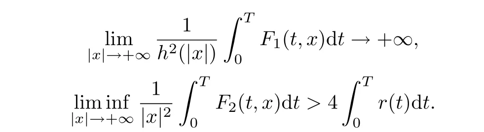
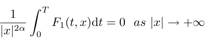
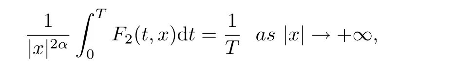
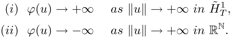
Theorem 1 Suppose that F = F1+F2satisfies assumption (A), (F1), (F2), and the following condition:(V1) there exists a nonnegative function h ∈C([0,+∞),[0,+∞))which satisfies the conditions(i)?(iv) and

Then problem (1.1) has at least one solution in

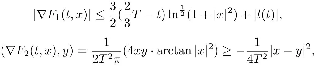
Remark 1 Theorem 1 extends Theorem 1.2 in[19],in which it is special case of Theorem 1 with control function h(t) = tα, α ∈[0,1), t ∈[0,+∞). What’s more, there are functions F(t,x)=F1(t,x)+F2(t,x) satisfy our theorems and do not satisfy the results in [5,7,12,13,16-22]. For example, let

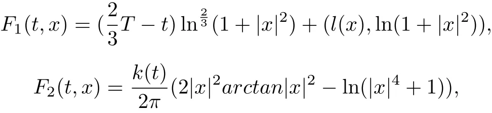
where l(t)∈L1(0,T;RN), k(t)We have

for any α ∈[0,1), and

so this example cannot be solved by theorem 1.2 [19], theorem 1.1 [22]and earlier results, such as [5, 7, 12-13, 16-22]. On the other hand, take h(|x|) =it is not difficult to see that (i), (iii) and (iv) of (F1) hold, and let C0=2, then

(ii) of (F1) holds. Moveover,

Remark 2Theorem 1 extends Theorem 1.1 in [13], in which it is a special case of our Theorem 1 corresponding to F2≡0.

Theorem 2Suppose that F = F1+F2satisfies assumption (A), (F1), (F2), and the following condition:

(V2) there exists a nonnegative function h ∈C([0,+∞),[0,+∞)) which satisfies the conditions (i)?(iv) and

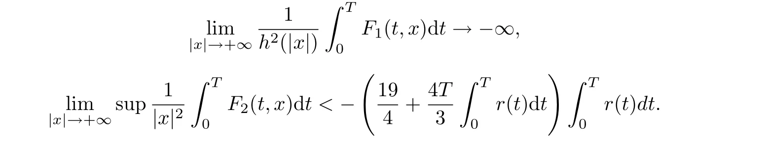
Then problem (1.1) has at least one solution in

Remark 3We note that Theorem 2 generalizes Theorem 1.2 in[13], which is the special case of our Theorem 2 corresponding to F2≡0.

Theorem 3Suppose that F = F1+ F2satisfies assumption (A), (F1), (F2), (V2).Assume that there exist δ >0,0 and an integer k >0 such that

for all x ∈RNand a.e. t ∈[0,T], and

for all |x| ≤δ and a.e. t ∈[0,T], where wThen problem (1.1) has at least two distinct solution in

Theorem 4Suppose that F = F1+ F2satisfies assumption (A), (F1), (F2), (V1).Assume that there exist δ >0,0 and an integer k >0 such that

for all |x|≤δ and a.e. t ∈[0,T], where w =Then problem (1.1) has at least three distinct solution in

§2. Preliminary Results

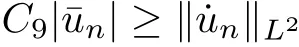
Proposition 2.1[5,Proposition1.1]There exists c>0 such that, if u ∈H1T, then

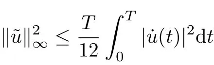
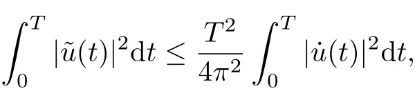
Proposition 2.2[5,Proposition1.3]If u ∈andu(t)dt=0, then

( Wirtinger’s inequality ) and

(Sobolev inequality).

Lemma 2.3[5,Theorem1.1]If ? is weakly lower semi-continuous on a reflexive Banach space X and has a bounded minimizing sequence, then ? has a minimum on X.Lemma 2.4[5,Corollary1.1]Let L:[0,T]×RN×RN→R be defined by

where F :[0,T]×RN→R,is measurable in t for each x ∈RN, continuously differentiable in x for almost every t ∈[0,T]and satisfy the following conditions:

for a.e.t ∈[0,T], all x ∈RN, some a ∈C(R+,R+), and some b ∈L1(0,T;R+). If u ∈is a solution of the corresponding Euler equation)=0, then ˙u has a weak derivative ¨u and

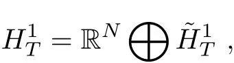
Lemma 2.5[3,Theorem4.6]Let E =where E is a real Banach space and Vand is finite dimensional, Suppose ? ∈C1(E,R), satisfies (PS)-condition, and(?1) there is a constant α and a bounded neighborhood D of 0 in V such thatand(?2) there is a constant β >α such that ?|X≤β.Then ? possesses a critical value c ≥β. Moreover c can be characterized as

where

Lemma 2.6[14,Theorem4]Let X be a Banach space with a direct sum decompositionwith dim X2< ∞, and let ? be a C1function on X with ?(0) = 0, satisfying(PS)-condition. Assume that some R>0,

and

Again, assume that ? is bounded from below and inf ?<0. Then ? has at least two non-zero critical points.

§3. Existence of Solutions

In this section we give the proofs of the main results.

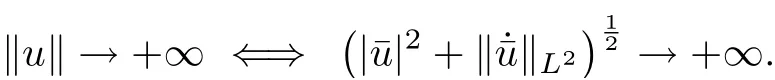
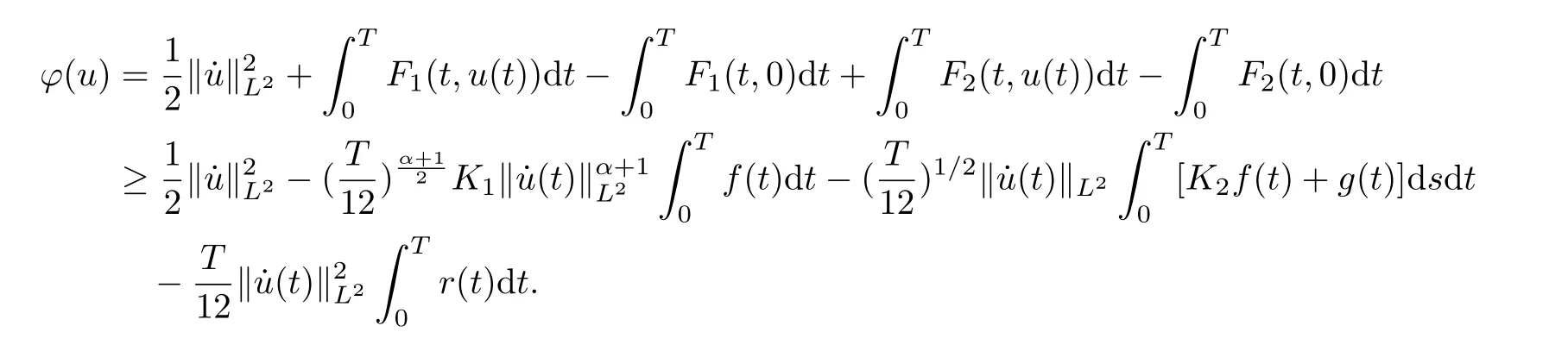
For convenience,we will denote various positive constants as Ci, i=1,2,3,···. For u ∈H1T,letdt and, then one has

and

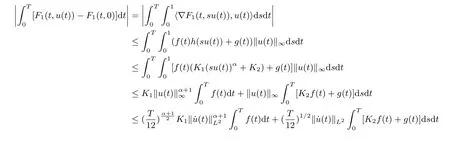
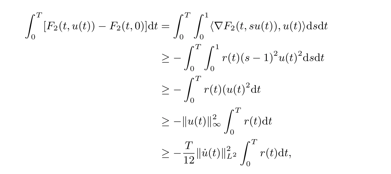
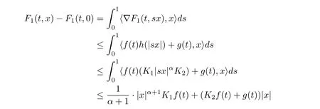
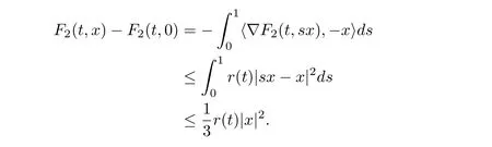
Proof of Theorem 1For u ∈H1T, it follows from (H1) and sobolev’s inequality that

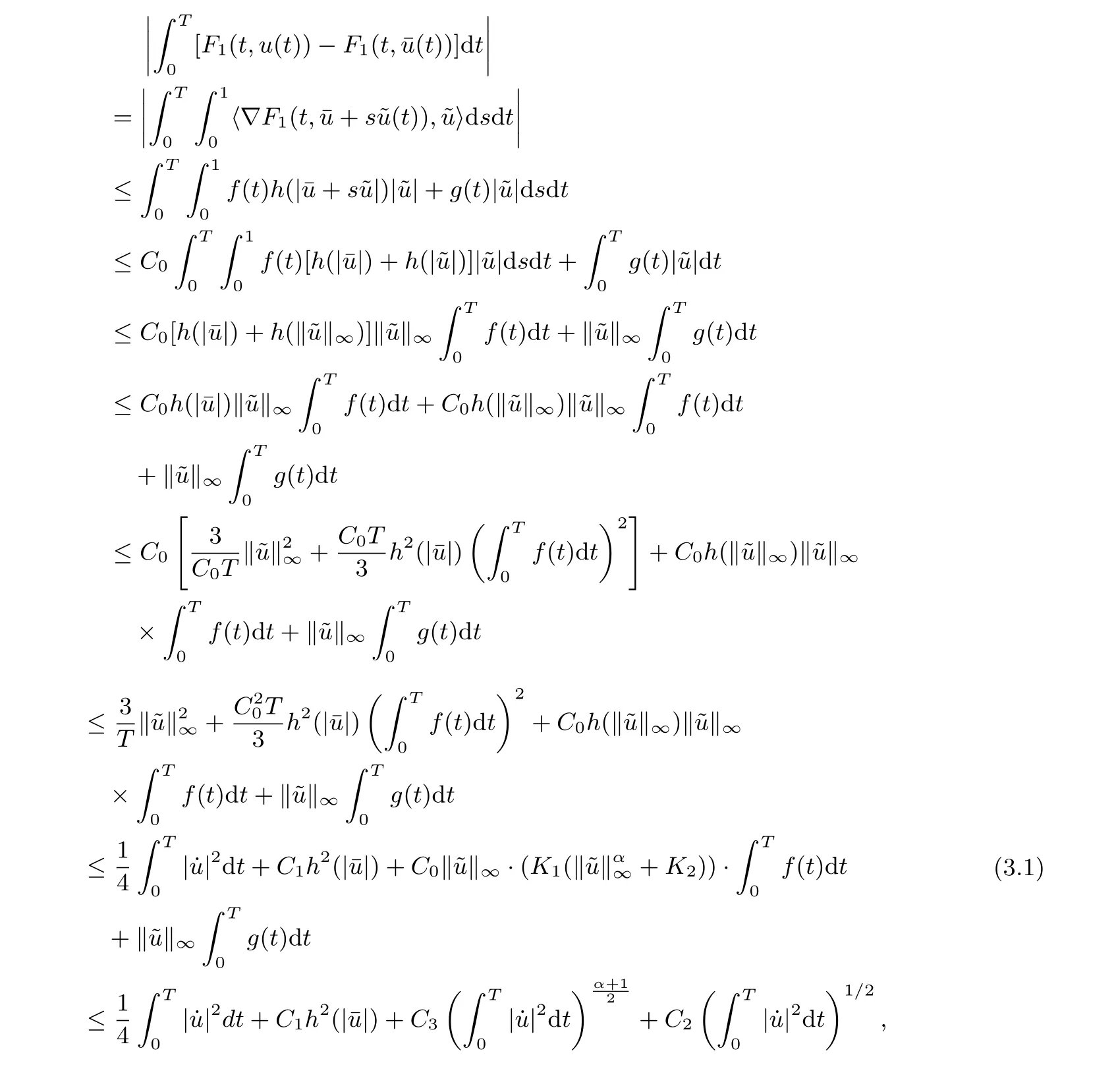
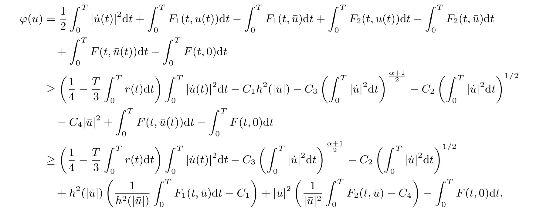
Note that

Then by condition (V1), and the fact thatone has

Since ? is weakly lower semi-continuous onby lemma 2.3 and lemma 2.4[5]the result holds.

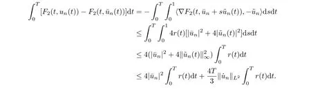
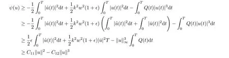
Proof of Theorem 2Step 1. We prove that ? satisfies the(PS)condition. Assume thatis a (PS) sequence for ?, that is,→0 as n →+∞and ?(un) is bounded,for n large enough, suppose thatDefine un=as before. For all u ∈by Proposition 2.1 and Proposition 2.2, one has

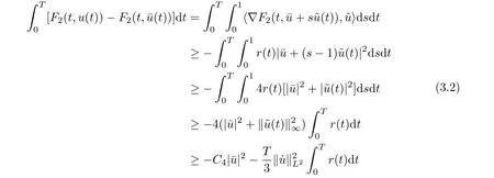
Then, by condition (F1) and the above inequality, we have

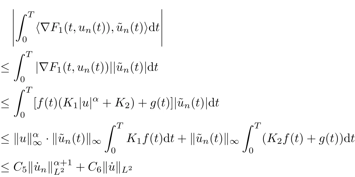
for some positive constants C5, C6. By condition (F2) and the sobolev’s inequality, one has

Hence, we see that

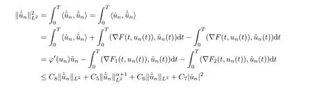
for large n and some positive condition C8.

By the above inequality, thus we obtain

for some C9and large n due to α<1. By condition (F2) and the Sobolev inequality, we have

By (3.1), the above inequality and the boundedness of {?(un)},

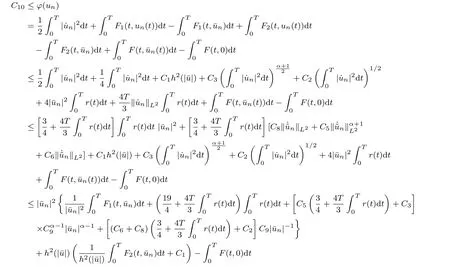
for some positive constant C10, by (V2), which implies that

it is in contradiction with the boundedness of{?(un)},so{ˉun}is bounded,thus{un}is bounded too. Arguing then as in proposition 4.1 in [5], {ˉun} has a convergent subsequence which shows that the (PS) condition holds.

Step 2. We prove that ? satisfies the rest conditions of the lemma 2.5. Suppose that

which implies that

By Wirtinger’s inequality, one has

Hence, (i) holds.

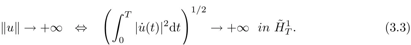
On the other hand, by (V2), we obtain

Combine (3.3) and (3.4), applying Lemma 2.5, then problem (1.1) has at least one solution in

Proof of Theorem 3Let E =

and ψ = ??. Then ψ ∈C1(E,R) satisfies the (PS) condition by the proof of Theorem (1.2).

In view of theorem 5.29 and Example 5.26 in [3], we only need to prove that

(ψ1) lim inf>0 as u → 0 in Hk,

(ψ2) ψ(u)≤0 for all u inand

(ψ3) ψ(u)→?∞as→∞in

In fact, by (F1), (F2), one has

and

We see that

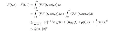
for all x ∈RNand a.e. t ∈[0,T], for all|x|≥δ, a.e. t ∈[0,T]and some Q ∈L1(0,T;R+)given by

Now it follows from (1.5) that

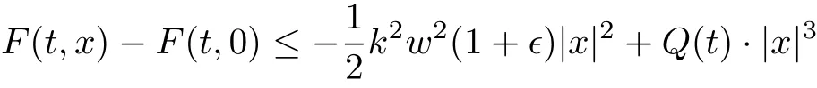
for all x ∈RNa.e. t ∈[0,T]. Moreover, for all u ∈Hk, it satisfies u=where=0,cos jwt+bjsinwt), and

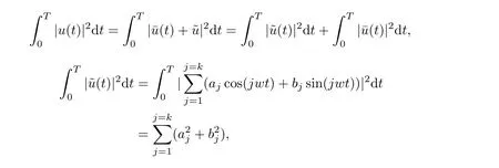
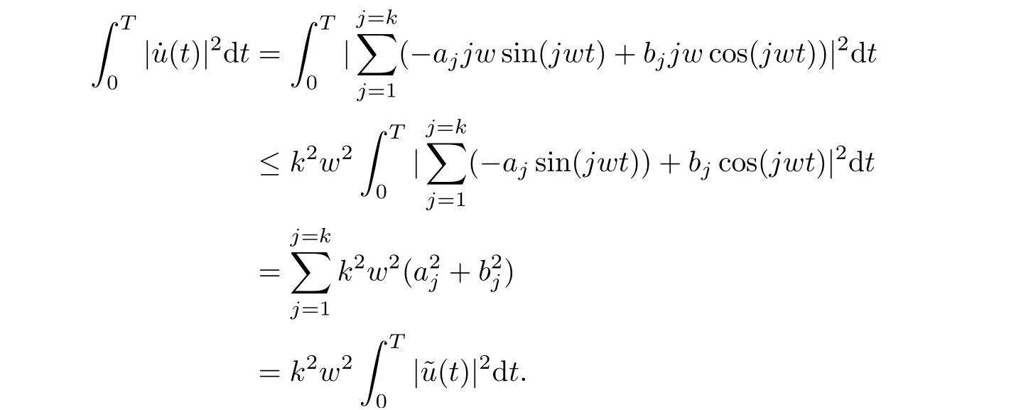
Hence we obtain

for all u ∈Hk, whereand C is a positive constant such that

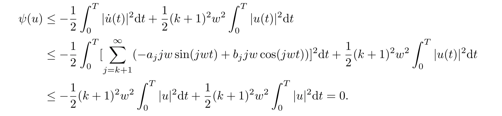
so(ψ2)is obtained. At last(ψ3)follows from(3.3). Hence the proof of theorem 1.3 is completed.

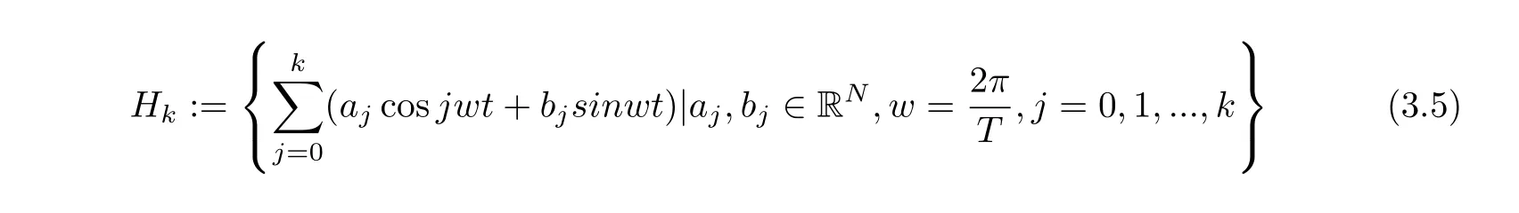
Proof of Theorem 4From the proof of Theorem 1.1, we know that ? is coercive which implies the (PS) condition. Let X2be the finite-dimensional subspace Hkgiven by (3.5) and let X1=. Then by (1.6) we have

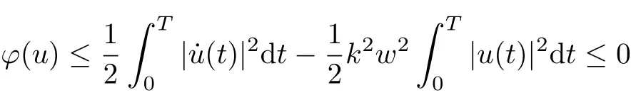
for all u ∈X2with≤C?1δ and

for all u ∈X1with≤C?1δ, where C is the positive constant given in (3.6).

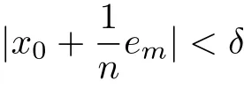
for every given |x|<δ, implies inf ?<0. Now our Theorem 4 follows from Lemma 2.6.

Then measE(x)=0 for all |x|<δ. Given |x|<δ we have