
BOUNDEDNESS OF VARIATION OPERATORS ASSOCIATED WITH THE HEAT SEMIGROUP GENERATED BY HIGH ORDER SCHRDINGER TYPE OPERATORS?
2020-11-14 09:40:34SuyingLIU劉素英
關(guān)鍵詞:張超
Suying LIU (劉素英)
Department of Applied Mathematics, Northwest Polytechnical University, Xi’an 710072, China
E-mail : suyingliu@nwpu.edu.cn
Chao ZHANG (張超)?
School of Statistics and Mathematics, Zhejiang Gongshang University, Hangzhou 310018, China
E-mail : zaoyangzhangchao@163.com
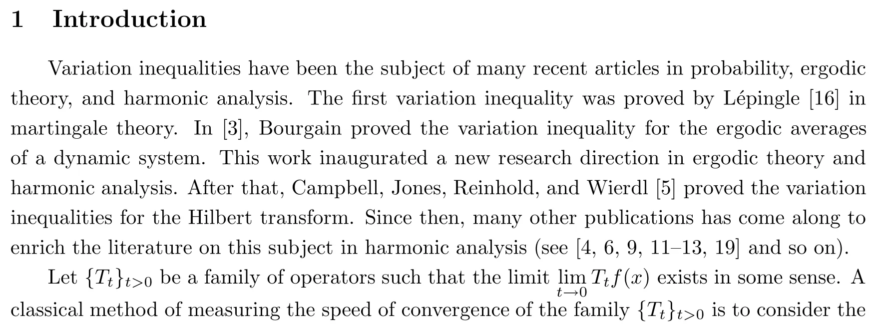
“square function” of the typewhere ti0, or more generally the variation operator Vρ(Tt), where ρ >2, is given by

where the supremum is taken over all the positive decreasing sequences{tj}j∈Nwhich converge to 0. We denote with Eρthe space including all the functions w :(0,∞)→ R such that
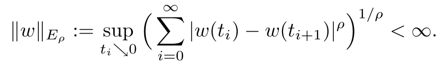
wEρis a seminorm on Eρ; it can be written as

In this article, we mainly focus on the variation operators associated with the high order Schrdinger type operators L=(??)2+V2in Rnwith n ≥ 5,where the nonnegative potential V belongs to the reverse Hlder class RHqfor some q > n/2; that is, there exists C > 0 such that
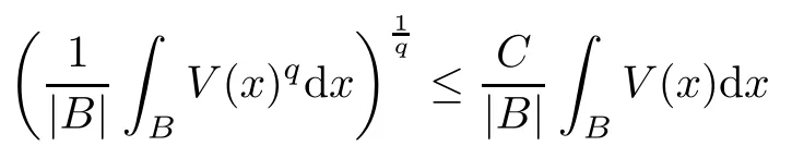
for every ball B in Rn. Some results related to(??)2+V2were first considered by Zhong in[29].In [25], Sugano proved the estimation of the fundamental solution and the Lp-boundedness of some operators related to this operator. For more results related to this operator,see[7,17,18].
The heat semigroup e?tLgenerated by the operator L can be written as

The kernel of the heat semigroup e?tLsatisfies the estimate

for more details see [1].
We recall the definition of the function γ(x), which plays an important role in the theory of operators associated with L:

This was introduced by Shen [21].
Theorem 1.1Assume that V ∈ RHq0(Rn), where q0∈ (n/2,∞) and n ≥ 5. For ρ > 2,there exists a constant C >0 such that

We should note that our results are not contained in the article of Bui [4], because the estimates of the heat kernel are not the same.
On the other hand, Zhang and Wu [28]studied the boundedness of variation operators associated with the heat semigroup {e?tL}t>0on Morrey spaces related to the non-negative potential V. Tang and Dong [26]introduced Morrey spaces related to non-negative potential V for extending the boundedness of Schrdinger type operators in Lebesgue spaces.
Definition 1.2Let 1 ≤ p < ∞,α ∈ R, and 0 ≤ λ < n. Forand V ∈RHq(q >1), we say that
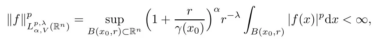
where B(x0,x) denotes a ball centered at x0and with radius r and γ(x0) is defined as in (1.2).
For more information about the Morrey spaces associated with differential operators, see[10, 23, 27].
We can now also obtain the boundedness of the variation operators associated to the heat semigroup {e?tL}t>0on Morrey spaces.
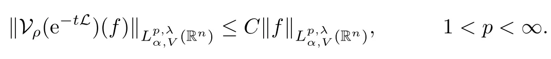
Theorem 1.3Let V ∈ RHq0(Rn) for q0∈ (n/2,∞), n ≥ 5, and ρ > 2. Assume that α ∈ R and λ ∈ (0,n). There exists a constant C >0 such that
The organization of the article is as follows: Section 2 is devoted to giving the proof of Theorem 1.1. In order to prove this theorem, we should study the strong Lp-boundedness of the variation operators associated with {e?t?2}t>0first. We will give the proof of Theorem 1.3 in Section 3. We also obtain the strong Lp(Rn) estimates (p > 1) of the generalized Poisson operatorson Lpspaces as well as Morrey spaces related to the non-negative potential V,in Sections 2 and 3, respectively.
Throughout this article, the symbol C in an inequality always denotes a constant which may depend on some indices, but never on the functions f under consideration.
2 Variation Inequalities Related to {e?tL}t>0 on Lp Spaces
In this section, we first recall some properties of the biharmonic heat kernel. With these kernel estimates,we will give the proof of Lp-boundedness properties of the variation operators related to {e?t?2}t>0, which is crucial in the proof of Theorem 1.1.
2.1 Biharmonic heat kernel
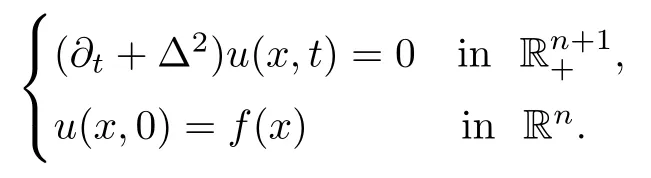
Consider the following Cauchy problem for the biharmonic heat equation:
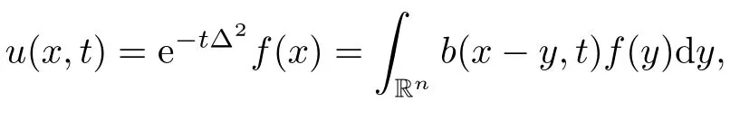
Its solution is given by
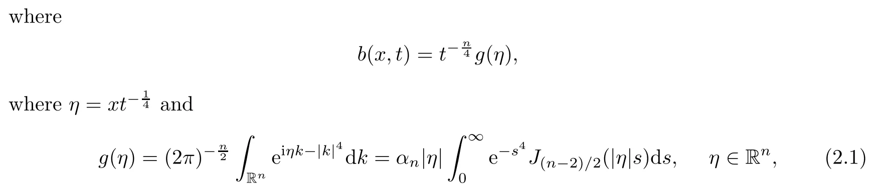
where Jvdenotes the v-th Bessel function and αn>0 is a normalization constant such that
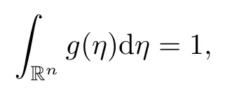
and g(η) satisfies the following estimates
see [14]. Then, by classical analysis, we have the following results (for details, see [24]):
(a) If f ∈ Lp(Rn), 1 ≤ p ≤ ∞, then
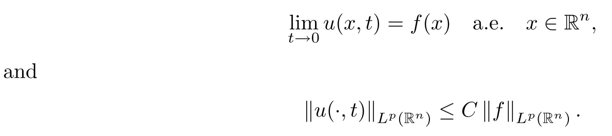
(b) If 1 ≤ p< ∞, then

We should note that the heat semigroup e?t?2does not have the positive preserving property; that is,when f ≥ 0, e?t?2f ≥ 0 may not to be established. Thus,the boundedness of the variation operators associated with {e?t?2}t>0cannot be deduced by the results in [11].
For the heat kernel b(x,t) of the semigroup e?t?2, we have the following estimates:
Lemma 2.1For every t>0 and Rn, we have
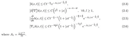
ProofFor (2.3) and (2.4), see Lemma 2.4 in [14]. From (2.1), (2.2), and some simple calculations, we can derive (2.5) and (2.6).
2.2 Variation inequalities related to {e?t?2}t>0
By Lemma 2.1 in Section 2.1, we know that the operator e?t?2is a contraction on L1(Rn)and L∞(Rn). Thus, e?t?2is contractively regular. Then, by [15, Corollary 3.4], we have the following theorem (for more details, see [15]):
Theorem 2.2For ρ>2, there exists a constant C >0 such that

2.3 Variation inequalities related to {e?tL}t>0
First, we recall some properties of the auxiliary function γ(x), which will be used later.
Lemma 2.3([21]) Let VThen there exist C and k0> 1 such that for all x,y ∈Rn,
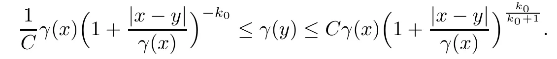
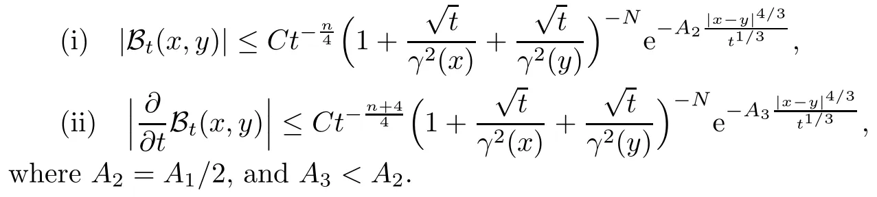
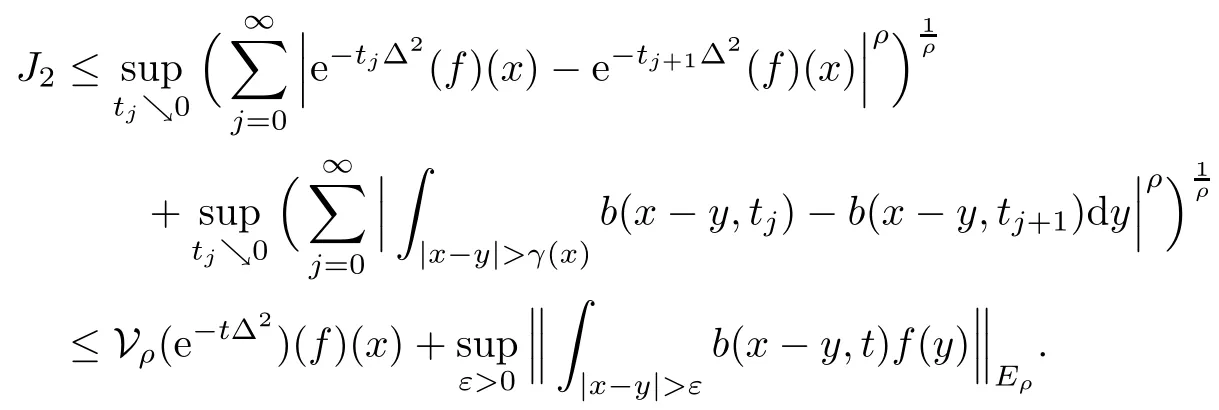
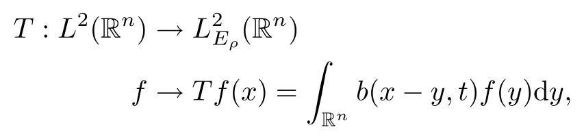
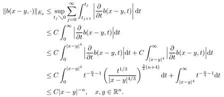
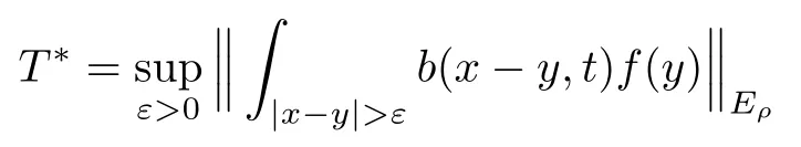
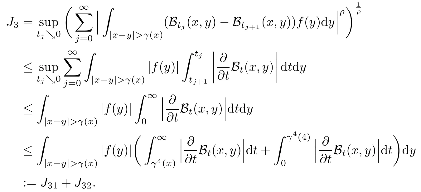
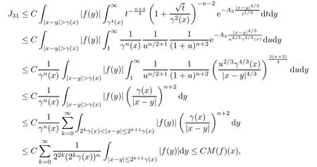
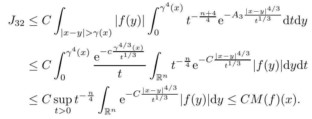
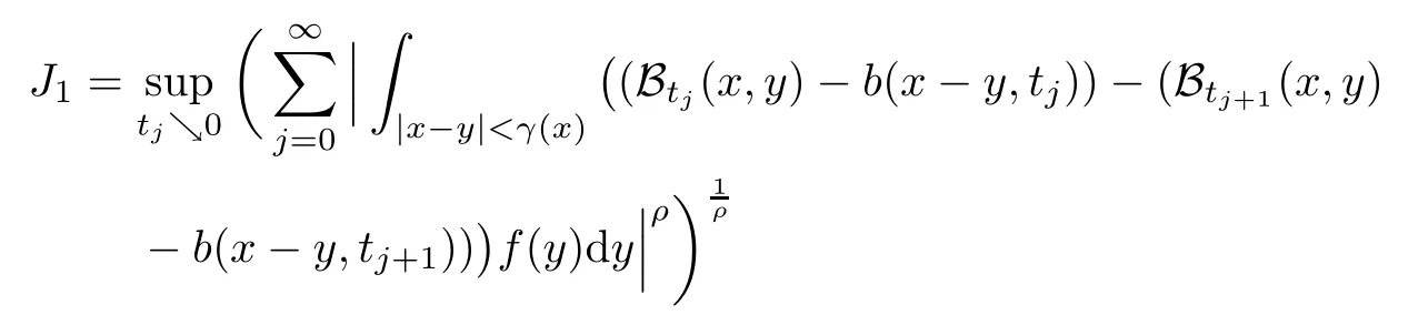
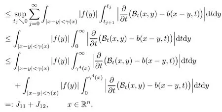
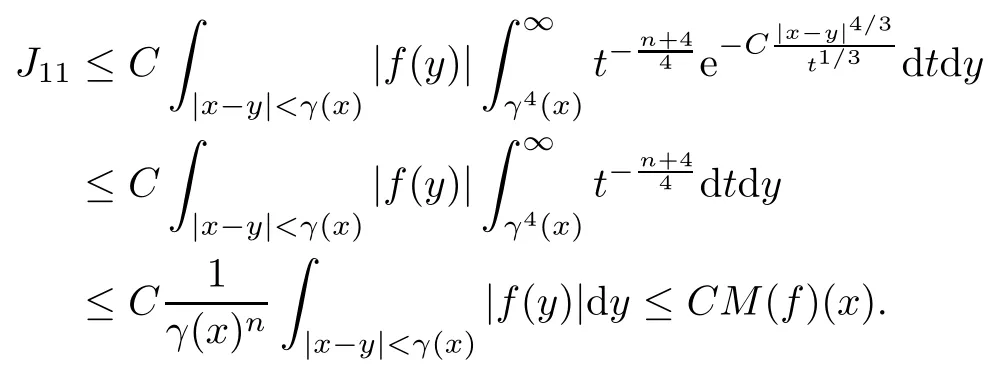
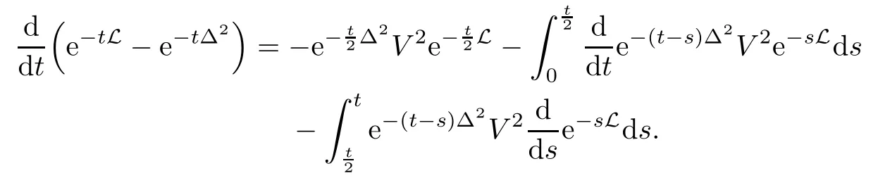
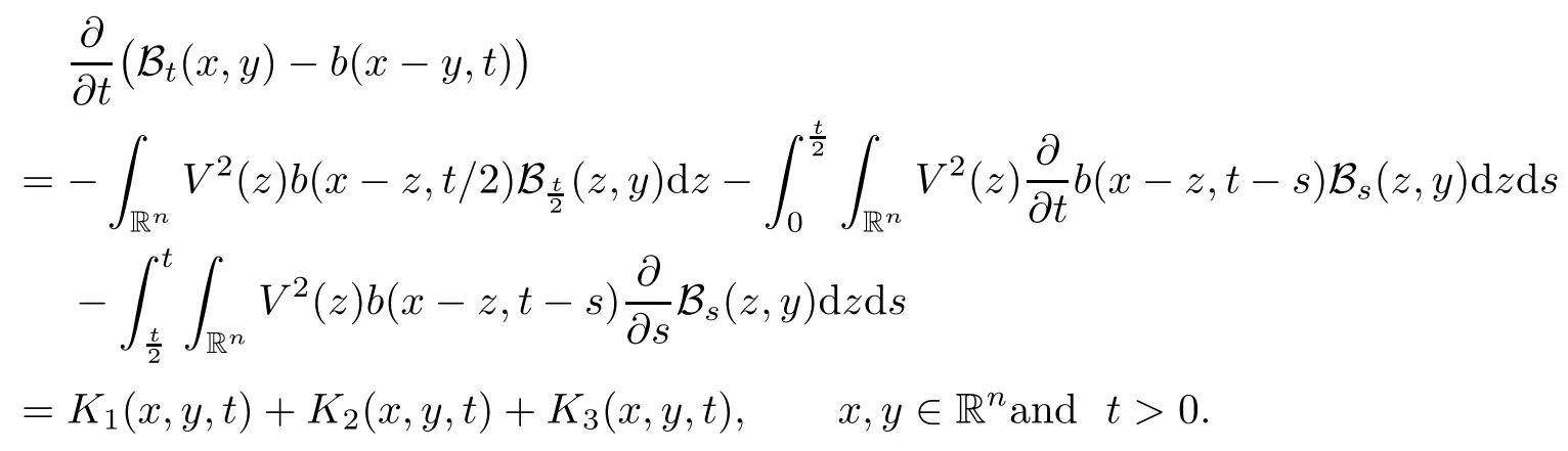
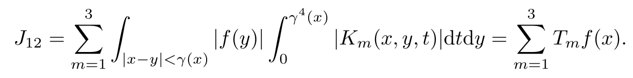
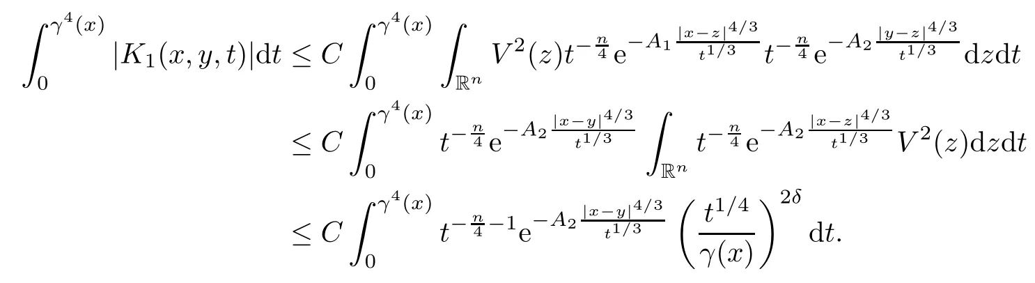
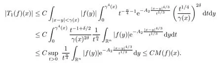
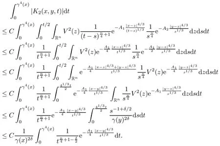
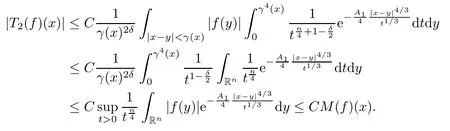
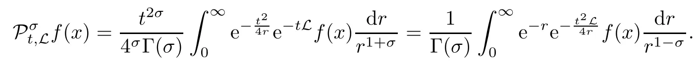
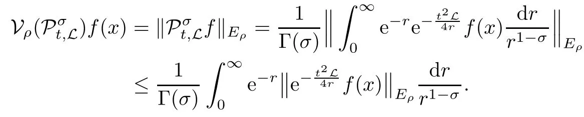
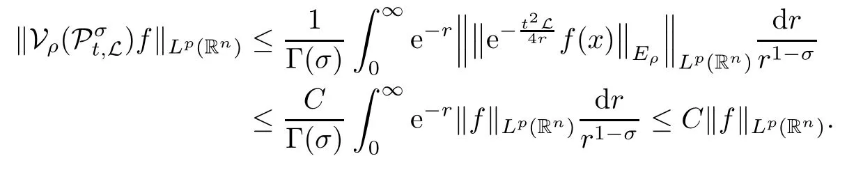
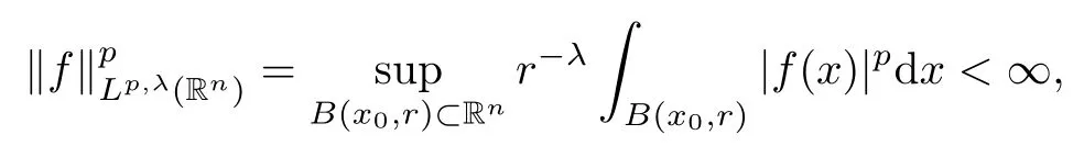
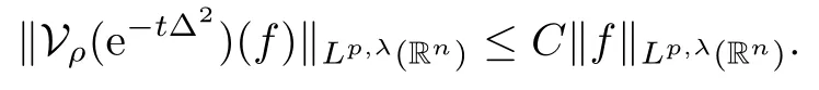
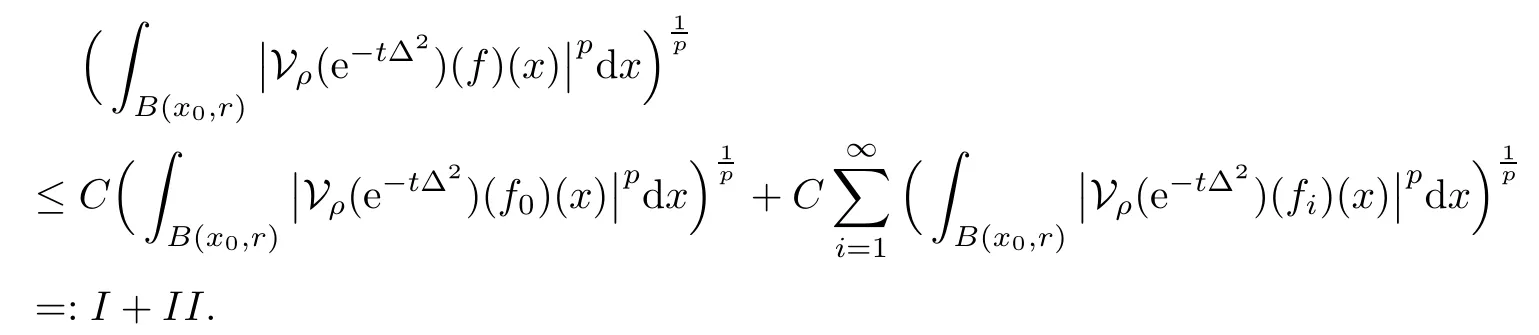
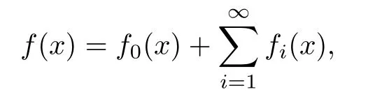
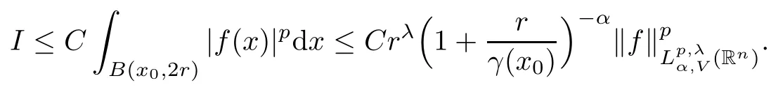
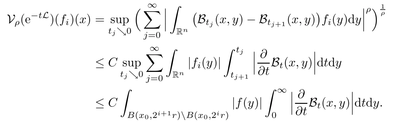
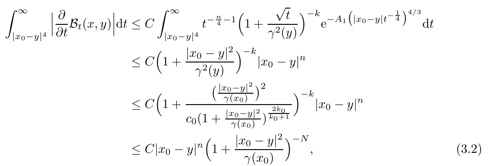
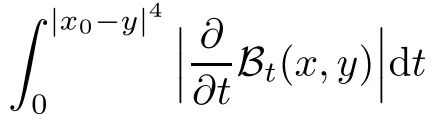
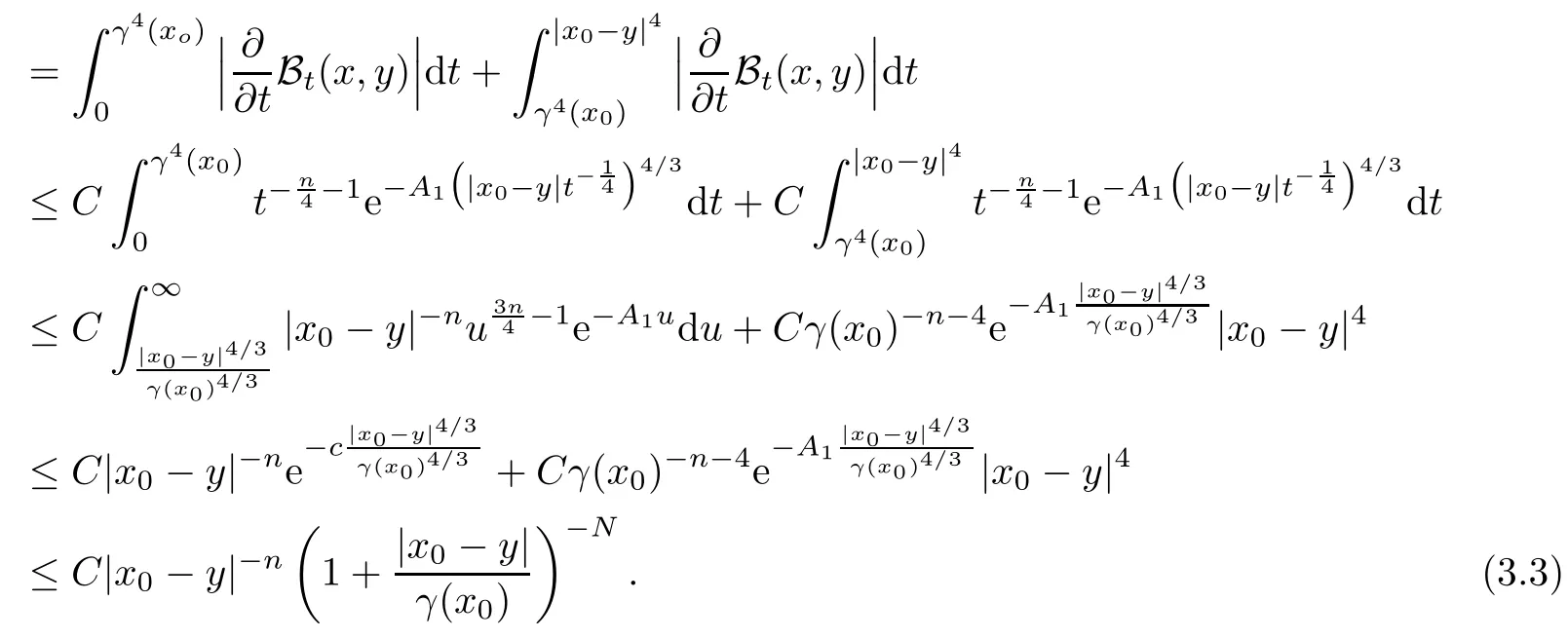
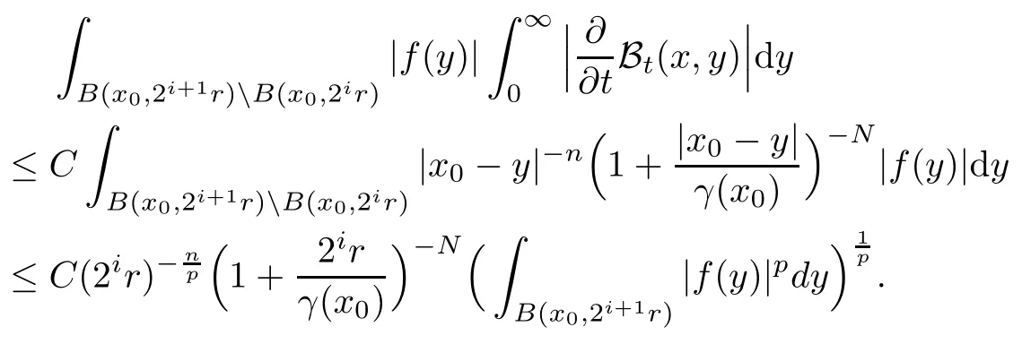
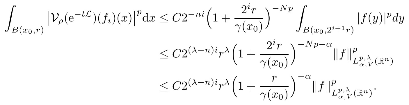
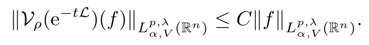
In particular, γ(x)~ γ(y) if |x ? y| Lemma 2.4(Lemma 2.7 in[7]) Let V ∈ RHq0(Rn)and δ =2?n/q0,where q0∈ (n/2,∞)and n ≥ 5. Then there exists a positive constant C such that for all x,y ∈ Rnand t ∈ (0,γ4(x)], where A4=min{A,A1} and A,A1are constants as in (1.1) and (2.3), respectively. Now we can prove the following kernel estimates of e?tL: Lemma 2.5For every N ∈N, there exist positive constants C, A2, and A3such that for all x,y ∈ Rnand 0 ProofFor (i), see Theorem 2.5 of [7]. Now we give the proof of (ii). As L = (??)2+V2is a nonnegative self-adjoint operator,we can extend the semigroup {e?tL} to a holomorphic semigroup {Tξ}ξ∈?π/4uniquely. By a similar argument as to that in [8, Corollary 6.4], the kernel Bξ(x,y) of Tξsatisfies The Cauchy integral formula combined with (2.7) gives Thus, we complete the proof. With the estimates above, we can give the proof of Theorem 1.1. Proof of Theorem 1.1For f ∈ Lp(Rn),1 ≤ p< ∞, we consider the local operators Then, we have Let us analyze term J2first: Now, we consider the operator defined by which is bounded from L2(Rn) intoaccording to Theorem 2.2. Moreover, T is a Caldern-Zygmund operator with the Eρ-valued kernel b(x?y,t). In fact, the kernel b(x?y,t)has the following two properties: (A) By (2.5), we have (B) Proceeding a similar way, together with (2.4), we have Thus, by proceeding as in the proof of [22, Proposition 2 in p.34 and Corollary 2 in p.36],we can prove that the maximal operator T?defined by is bounded on Lp(Rn) for every 1 < p < ∞. Combining this with Theorem 2.2, we conclude thatis bounded from Lp(Rn) into itself for every 1 Next, we consider term J3: To estimate J31, by Lemma 2.5 with N =n+2 and changing variables, we have where M(f) is the Hardy-Littlewood maximal function of f. For J32, by Lemma 2.5, we have Thus,from the estimates J31and J32,we have J3≤CM(f)(x),which implies that the operatoris bounded from Lp(Rn) into itself for every 1 Finally, we consider the term J1: Applying Lemma 2.1 and Lemma 2.5, we have The formula (2.7) in [7]implies that Then we have We rewrite J12as Using (2.3), and Lemmas 2.5 and 2.4, we obtain As a consequence, Next, we note that when 0 Hence, As in the previous proof, proceeding with a similar computation, we can also obtain Owing to the above estimates, we know that J12≤ CM(f)(x). Consequently, we have J1≤CM(f)(x). As M(f) is bounded from Lp(Rn) into itself for every 1 < p < ∞, the proof of Theorem 1.1 is complete. For 0< σ <1, the generalized Poisson operatorassociated with L is defined as For the variation operator associated with the generalized Poisson operatorswe have the following theorem: Theorem 2.6Assume that V ∈ RHq0(Rn), where q0∈ (n/2,∞) and n ≥ 5. For ρ > 2,there exists a constant C >0 such that1 ProofWe note that Then, for 1 In this section, we will give the proof of Theorem 1.3. For convenience, we first recall the the definition of classical Morrey spaces Lp,λ(Rn), which were introduced by Morrey [20]in 1938. Definition 3.1Let 1 ≤ p< ∞, 0 ≤ λ < n. Forwe say that f ∈ Lp,λ(Rn)provided that where B(x0,r) denotes a ball centered at x0and with radius r. In fact, when α = 0 or V = 0 and 0< λ < n, the spaceswhich were defined in Definition 1.2, are the classical Morrey spaces Lp,λ(Rn). We establish the Lp,λ(Rn)-boundedness of the variation operators related to{e?t?2}t>0as follows: Theorem 3.2Let ρ>2 and 0<λ ProofFor any fixed x0∈Rnand r > 0, we write f(x) =where f0 =fχB(x0,2r), fi =fχB(x0,2i+1r)B(x0,2ir) for i ≥ 1. Then For I, by Theorem 2.2, we have For II, we first analyze Vρ(e?t?2)(fi)(x). For every i ≥ 1, Note that for x ∈ B(x0,r) and y ∈ RnB(x0,2r), we know thatBy using(2.5), we have The proof of this theorem is complete. The following is devoted to the proof of Theorem 1.3. Proof of Theorem 1.3Without loss of generality, we may assume that α<0. Fixing any x0∈Rnand r >0, we write where f0=fχB(x0,2r), fi=fχB(x0,2i+1r)B(x0,2ir)for i ≥ 1. Then From (i) of Theorem 1.1, we have For II, we first analyze Vρ(e?tL)(fi)(x). For every i ≥ 1, Note that for x ∈ B(x0,r) and y ∈ RnB(x0,2r), we have |x ? y| >We discussin two cases. For the one case, |x0?y|≤ γ(x0), by(ii) of Lemma 2.5 we have For the other case, |x0? y| ≥ γ(x0), applying (ii) of Lemma 2.5 together with Lemma 2.3 we have Combining (3.1), (3.2) and (3.3), we have Thus, taking N =[?α]+1, we obtain The proof of the theorem is completed. Finally, we can give the boundedness of the variation operators related to generalized Poisson operatorsin the Morrey spaces as follows: Theorem 3.3Let V ∈ RHq0(Rn) for q0∈ (n/2,∞), n ≥ 5, and ρ > 2. Assume that α ∈ R and λ ∈ (0,n). There exists a constant C >0 such that ProofWe can prove this theorem by the same procedure used in the proof of Theorem 2.6.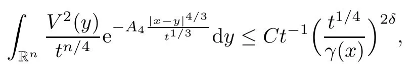


2.4 The generalized Poisson operators
3 Variation Inequalities on Morrey Spaces


 猜你喜歡
當代美術(shù)家(2023年4期)2023-08-04 23:34:30散文百家(2021年11期)2021-11-12 03:06:38中學生英語·中考指導版(2021年12期)2021-09-27 09:20:45中學生英語·中考指導版(2021年1期)2021-05-17 03:25:04散文百家(2021年4期)2021-04-30 03:15:20散文百家(2021年2期)2021-04-03 14:08:22攝影與攝像(2020年7期)2020-09-10 07:22:44美與時代·美術(shù)學刊(2019年9期)2019-11-29 13:17:39數(shù)學大王·低年級(2019年9期)2019-10-09 03:39:52中學生英語·閱讀與寫作(2019年12期)2019-01-17 04:54:51
猜你喜歡
當代美術(shù)家(2023年4期)2023-08-04 23:34:30散文百家(2021年11期)2021-11-12 03:06:38中學生英語·中考指導版(2021年12期)2021-09-27 09:20:45中學生英語·中考指導版(2021年1期)2021-05-17 03:25:04散文百家(2021年4期)2021-04-30 03:15:20散文百家(2021年2期)2021-04-03 14:08:22攝影與攝像(2020年7期)2020-09-10 07:22:44美與時代·美術(shù)學刊(2019年9期)2019-11-29 13:17:39數(shù)學大王·低年級(2019年9期)2019-10-09 03:39:52中學生英語·閱讀與寫作(2019年12期)2019-01-17 04:54:51
 Acta Mathematica Scientia(English Series)2020年5期