
EXPONENTIAL STABILITY OF A MULTI-PARTICLE SYSTEM WITH LOCAL INTERACTION AND DISTRIBUTED DELAY*
2022-11-04 09:07:24
College of Liberal Arts and Sciences,National University of Defense Technology,Changsha 410073,China
E-mail: liuyc2001@hotmail.com
Abstract For a collective system,the connectedness of the adjacency matrix plays a key role in making the system achieve its emergent feature,such as flocking or multi-clustering.In this paper,we study a nonsymmetric multi-particle system with a constant and local cut-offweight.A distributed communication delay is also introduced into both the velocity adjoint term and the cut-offweight.As a new observation,we show that the desired multiparticle system undergoes both flocking and clustering behaviors when the eigenvalue 1 of the adjacency matrix is semi-simple.In this case,the adjacency matrix may lose the connectedness.In particular,the number of clusters is discussed by using subspace analysis.In terms of results,for both the non-critical and general neighbourhood situations,some criteria of flocking and clustering emergence with an exponential convergent rate are established by the standard matrix analysis for when the delay is free.As a distributed delay is involved,the corresponding criteria are also found,and these small time lags do not change the emergent properties qualitatively,but alter the final value in a nonlinear way.Consequently,some previous works [14] are extended.
Key words semi-simple eigenvalue;flocking emergence;clustering emergence;distributed delay;exponential convergence
1 Introduction
Self-organized collective systems arise very naturally in artificial intelligence,physical,biological and social sciences.Such systems have a remarkable capability to regulate the flow of information from distinct and independent components to achieve a prescribed performance.It is of particular interest,in terms of both theory and application,to understand how self propelled individuals use only limited environmental information and simple rules to organize themselves into an ordered motion.In terms the modelling and analysis frame,multi-particle models have been widely used to verify practical observations;see [2,14,28] and the references therein for examples.Our main motivation in the current work is to analyze and explain emergent patterns on a delayed particle model,while individual particles interact only locally and connectedness is also lost.
As we know,to gain ordered collective performance,there are three items would be included in modelling and qualitative analysis.One is symmetry,which means that the interactions between each pair of particle is the same.The second is global interaction for all individuals.The final item is the connectedness of the adjacency structure.Taking these things into consideration,the celebrated Cucker-Smale model [5,6],proposed in 2007,provided a framework for examining the emergent properties of flocks in order to explain self-organized behaviors in one kind of complex system.In successive contributions,non-symmetric interaction,local interaction weight and delay arguments were all incorporated in more general model settings.For more detailed discussions,we refer readers to [2,9,12–18,22,25,29] and the references therein.These works imply that the connectedness of the underlying adjacency matrix plays a crucial role in the analysis of synchronization.Naturally,removing the troublesome connectedness condition or finding the balance between local interaction and connectedness is a difficult problem,in theory.
In this paper,we consider anN-particle system with a distributed communication delay:
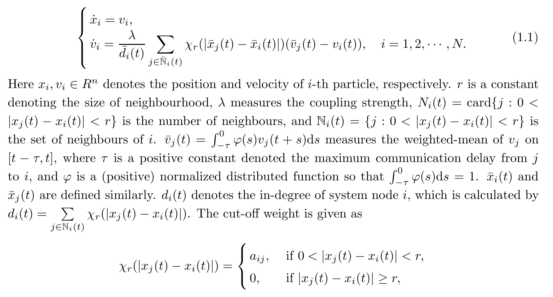
where the communication weightaijis selected from the candidate symmetric adjacency matrixA=(aij)N×N.Ifaij=1 for alli,j,thendi(t)=Ni(t).For more delayed collective models,see [2–4,7,8,11,19,23,24,27].
In particular,whenτ=0,this is a free delay forvj,i.e.,.Also,we have.Thus,the system (1.1) becomes
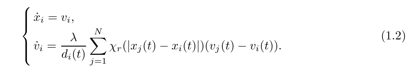
For the above equation,Jin [14] posted some criteria for achieving a flock when allaij=1.Whenris large enough,viwill be independent of |xi-xj|,and then system (1.1) degenerates into a first-order delayed system,as an opinion model;this was investigated by Atay in [1].
For our observations,the parameterris sensitive to the dynamics of system (1.2).Whenris small enough,each particle will be almost free of interaction from the others,and each particle evolves for itself uncertainly and strongly depends on its initial value.The dynamics of system (1.2) is complex in this case.Whenris large enough,each particle will interact with all of the others with the candidate adjacency matrixA.In this case,ifAis a connected matrix,then all particles achieve synchronization for arbitrary initial values.The dynamics of system (1.2) becomes simple.A natural question is: how do we verify the dynamical behaviors of system (1.1) when the distributed communication delay is involved? Our goal here is to give some new viewpoints regarding the dynamical behavior of system (1.1) when the connectedness of the adjacency matrix is absent and the distributed delay is involved.
The rest of this paper is organized as follows: in Section 2 we give more details for the model analysis and give some assumptions.In Section 3,for both the non-critical and general neighbourhood situations,some criteria regarding flocking and clustering emergence with an exponential convergent rate are established when the delay is free.In Section 4,when the distributed delay is involved,the criteria of flocking and clustering emergence are also found,and it is shown that these small time lags will not change the emergent property qualitatively,but alter the final value in a nonlinear way.
2 Preliminaries and Assumptions
2.1 Preliminaries
First,we give the mathematical definitions flocks and clusters.
Definition 2.1Suppose that (xi(t),vi(t)) ∈Rn×Rn(i=1,2,···,N) is a solution to(1.1).The above system is said to achieve a flock if

wherev∞∈Rnis a constant vector.
Definition 2.2Suppose that (xi(t),vi(t)) ∈Rn×Rn(i=1,2,···,N) is a solution to(1.1).The above system is said to achievep-clusters if there exist some vectorsφj∈Rnand setsSj?{1,2,···,N} satisfyingSj∩Si=? (empty set),φjφi(wheneverij) and∪jSj={1,2,···,N},such thatfor alli∈Sj,j=1,2,···,p.The numbersφj
are then called the clustering velocity.
To specify a solution for the multi-particle system (1.1),we need to specify the initial conditions

wherefiandgiare given continuous vector-value functions.
Also,to quantify the sensitivity of the adjacency matrix when the distance of two particles is nearr,we use the following variables ont:

lM(t)=max{lij(t): 1 ≤i,j≤N} andlm(t)=min{lij(t): 1 ≤i,j≤N} for allt >0.Naturally,we have Γ(t) ≥0.If Γ(t)>0,we call this case a non-critical neighbourhood situation.If Γ(t)=0,we call it general neighbourhood situation;see [14].
Define the adjacency matrix and average matrix byandP(t)=(pij(t))N×N,respectively,where
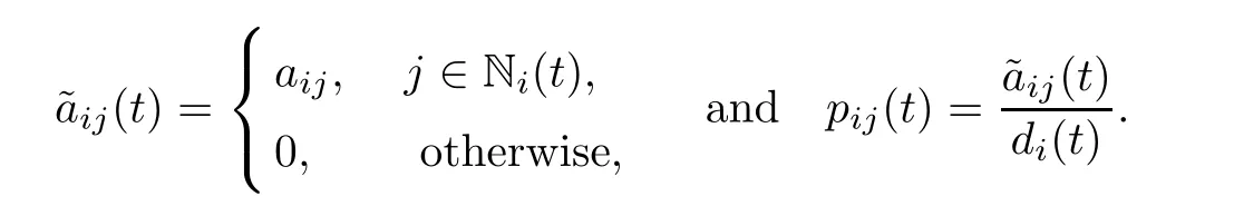
Recalling the matrix theory [26],a matrixS=(sij)N×Nis called stochastic ifsij≥0 and.The matrixSis said to be connected if,for arbitrary integersiandj(1 ≤i,j≤N),there are a sequence of integersk1,k2,···,kqsuch thatskl-1,kl>0,l=1,2,···,q+1,wherek0=i,kq+1=j.Noting that,from the above definitions,we see that the corresponding average matrixP(t) is a connected stochastic matrix.The matrixL(t)=I-P(t)is called the Laplacian matrix of the system (1.1).
Note that the average matrix will change when the distance from another particle is nearr.By the continuity of the trajectory ofxi(1 ≤i≤N),there existst1>0 such that the average matrixP(t) remains unchanged on [0,t1).Denotetnas the switching point at thenthtime.Then {tn} is called the switching point sequence,which can be finite or infinite.Since the average matrix remains unchanged at each interval (tn,tn+1),n=0,1,2,···,(t0=0),the matrixP(t) will be a constant matrix on (tn,tn+1),sayP(tn).In particular,setP(θ)=P0forθ∈[-τ,0].
In the sequel,we need the following vector norms: define
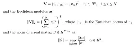
IfSis a square matrix,then ‖S‖ is the largest eigenvalue ofS.Using the above definitions and the Cauchy-Schwarz inequality,we see that

2.2 Assumptions
As we know,an eigenvalue is said to be semi-simple if its algebraic multiplicity equals its geometric multiplicity.Throughout the paper,we assume that 1 is a semi-simple eigenvalue of the matrixP0with algebraic multiplicityn0.Assume that the other eigenvalues ofP0areμ2,···,μm0,with the corresponding algebraic multiplicityp2,···,pm0,respectively.From the matrix theory,we see that |μi|<1 fori=2,···,m0,and there is a non-degenerate matrixT0such that,whereJ0is a diagonal matrix with the first block being 1,saywhere0is a zero matrix with a matchable dimension.Inspired by [14],we reset

ThenMis a symmetric matrix andPis similar toM.Therefore,Pis a diagonalizable matrix and all eigenvalues of matrixPare real.Also,there is an orthogonal matrixOsuch thatM0=OJ0O-1.Thus

Letdmax=max{d1(0),···,dN(0)} anddmin=min{d1(0),···,dN(0)}.Then the condition number of matrixP0has an upper bound,which reads as
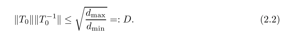
Without loss of generality,we assume that

Finally,to discuss the dynamical behaviors of system (1.1),we give the following assumptions:
(A1) Assume that the eigenvalue 1 of the initial average matrixP0is semi-simple and that the corresponding algebraic multiplicity isn0.
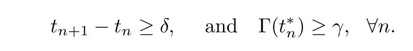
(A2) There exist positive constantsδ,γandsuch that
(A2τ) There exist positive constantsδ,γandsuch that

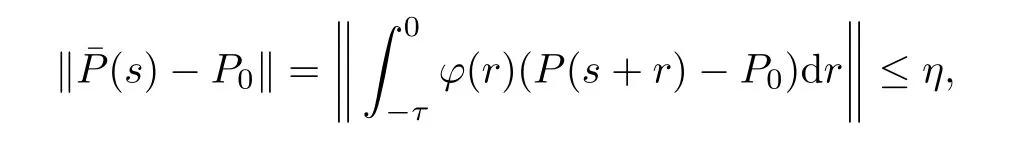
(A3) Assume that the amplitude ‖P(t) -P0‖ is bounded uniformly ont.Setη=
Remark 2.3Ifn0=1,then the matrixP0is a connected matrix,and whenevern0>1,the connectedness of matrixP0will be lost.
Remark 2.4To overcome the difficulty in the critical situation,we need that the average matrixP(t) does not change frequently and sharply.For this,we assume that all switching intervals have a uniform minimum gap in (A2) and (A2τ).Meanwhile,we assume that the average matrixP(t) admits a priori bound in (A3),although this depends on the dynamics of solutions.These assumptions are valid for making the designed system achieve a flock.
3 Convergence Analysis Without Delay Effects
As we know,the model (1.1) is a piecewise continuous system,and the successive system works with the initial values generated by the current system.In each continuous interval,model (1.1) is a linear system and has a unique solution.Thus,the solutions of model (1.1)have global existence and uniqueness.In this section,we focus on the convergence analysis of model (1.1) without delay effects.
LetX=(x1,x2,···,xN)Tand letV=(v1,v2,···,vN)T.Then system (1.2) becomes

Theorem 3.1Assume that (A1) holds,and that Γ(0)>0 and<λ(1 -μ2)Γ(0).Then

In particular,whenn0=1,system (1.2) achieves a flock.
ProofFrom the matrix theory and Assumption (A1),we see that there is a non-degenerate matrixT0such that
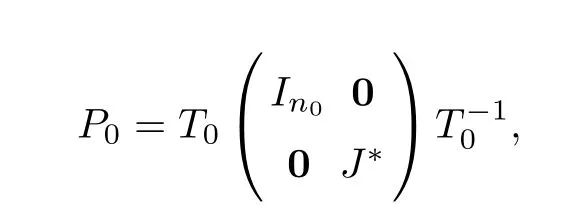
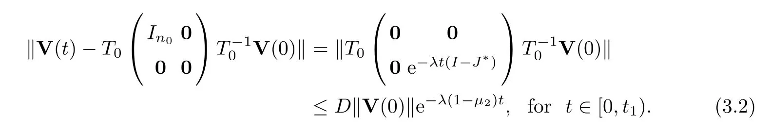
whereIn0is an0×n0identity matrix,andJ*is a Jordan block matrix.From equation (1.2),we have that
By direct computation,we obtain
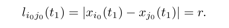
Next,we show thatt1=∞.Ift1<∞,then the average matrixP0will change att=t1.Thus,there exists (i0,j0) such that
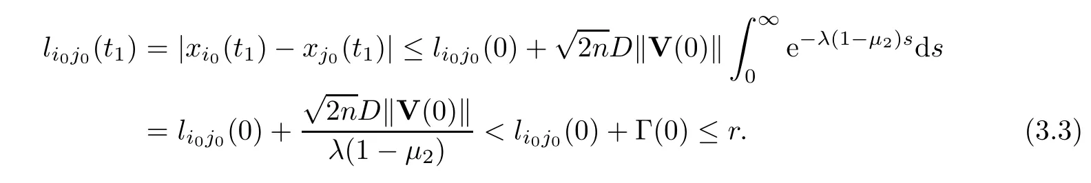
Case In0=1.Recalling the first equation of (1.2),we havei0(t)=vi0(t) and
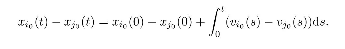
Thus,we get that
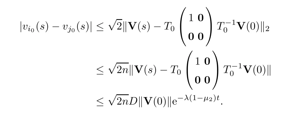
Thus,forj0∈Ni0(0),
On the other hand,forj0Ni0(0),
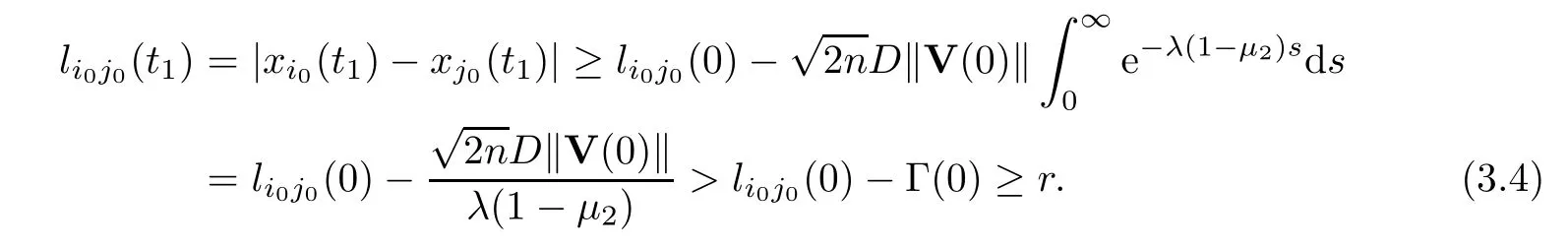
Obviously,the inequalities (3.3) and (3.4) contradict the fact that there exists (i0,j0),such thatli0j0(t1)=r.Thus,t1=∞andP(t) ≡P0for all time.
Case IIn0>1.Without loss of generality,if necessary,we exchange the rows of matrixP0and relabel the subscript ofvi.We assume thatP0is a block diagonal matrix;that is,P0=diag(Q1,Q2,···,Qn0) (see the details in Appendix A).In this case,we consider the subsystem

whereQiis also a stochastic matrix with a simple eigenvalue 1 fori=1,2,···,n0.Letμ2i=max{Rez: det(zI-Qi)=0,z1}.For,thek-th column ofP0is partially located inQi},and for,thek-th column ofP0is partially located inQi},so we have
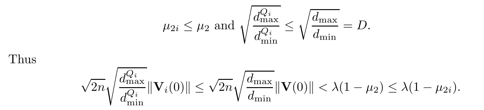
Since the eigenvalue 1 ofQiis simple,following similar arguments as to those in Case I,we conclude thatt1=∞.
Thus,from inequality (3.2),we have that
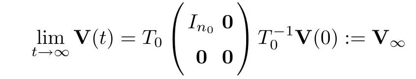

Next,we will verify that all of the components are the same.Indeed,recalling thatP0=,we assume that the first column ofT0is the vector (1,1,···,1)T.Letting
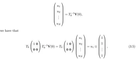
where ?denotes the Kronecker product.Thus,all of components are the same.

By Definition 1.1,system (1.2) achieves a flock whenn0=1.This completes the proof. □
Remark 3.2We remark that the final valueis independent of the choice ofT0.Indeed,takingT0=(c1,···,cn0,*) and,ri· ci=1 fori=1,2,···,n0.If we selectkici(ki0) as thei-th column ofT0,then thei-th row ofwould be.Then,
Thus,the final value is independent of the choice ofT0.
Remark 3.3In Theorem 3.1,ifn0=1 andaij=1,we obtain the results in Theorem 2.1 in [14].Thus Theorem 3.1 extends the corresponding results.
For whenn0>1,to understand the final collective performance,we give more details of.To this end,we have the following lemma:
Lemma 3.4([20],Lemma 3.2) Assume that zero is a semi-simple eigenvalue of the Laplacian L with multiplicityn0.Then there exists a unique family of normal zero-one vectorsa1,···,an0such thatLai=0 anda1+a2+···+an0=1.
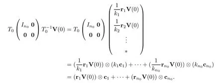
Recalling that each of the firstn0columns ofT0is the eigenvector of matrixI-P0with an eigenvalue 0,from Lemma 3.1 and setL=I-P0,we choose zero-one vectorsa1,···,an0as the firstn0columns ofT0,sayT0=(a1,···,an0,*).Lettinguibe thei-th component of

Since allaiare zero-one vectors,we see that the number of elements different from one and other in set {u1,u2,···,un0} will determine the number of clusters of system (1.1).Indeed,assume that the set {φ1,φ2,···,φk} consists of all elements different from one and other in set{u1,u2,···,un0}.Then
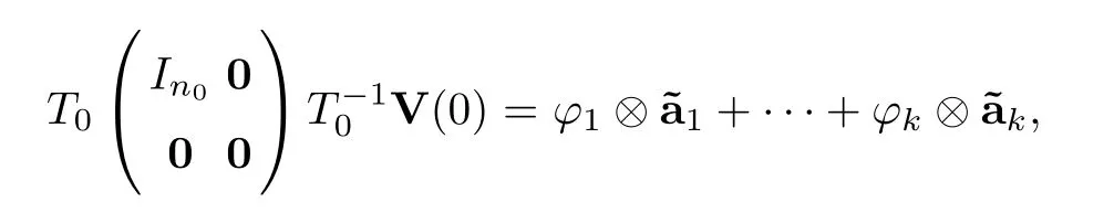
where1,···,kare zero-one vectors too.Let

Then ∪jSj={1,2,···,N} andfor alli∈Sj.Following Definition 1.2,system(1.2) achievesk-clusters.Thus we conclude with a following result.
Theorem 3.5Let (A1) hold and.Then the system (1.2)will achievek-clusters,wherekis the number of elements different from one and other in set{u1,u2,···,un0}.In particular,ifn0=1 orφ1=φ2=···=φk,then the system also achieves a flock.
3.1 Flocking and clustering analysis in a general situation
In this subsection,we focus on the general case in which the average matrixP(t) will change according to time.As we know,to make the designed systems of (1.2) achieve a prescribed flocking behavior,we need to assume that the average matrixP(t) does not change frequently and sharply.Also,the neighbouring particles do not stay in the critical situation (the neighbourhood of circle |xi-xj|=r) for a long time.For this,under the additional assumptions(A2) and (A3),we obtain similarly results in a noncritical situation.
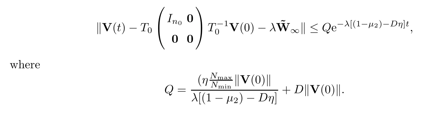
Theorem 3.6Assume that (A1),(A2) and (A3) hold,and thatDη <1 -μ2.Then the system is convergent with
and the convergent rate is given as
In particular,whenn0=1,the system achieves a flock.Whenn0>1,the system achieves a flock or multi-cluster.
ProofFirst,we rewrite system (1.2) as

By using the variation-of-constant formula,we have that
and recalling the fact that

we see that
whereηis given in Assumption (A3).That is,

By solving the above Gronwall’s inequality,we get that

Recalling the inequalityDη <1 -μ2,we find that there is a positive integral numberk0such that

whereγandδare as given in Assumption (A2).
Next,we show thattk0+1=∞.From Assumption (A2) again,there is a constant(tk0,tk0+1) such that.Indeed,iftk0+1<∞,then there exists (i0,j0) such thatli0j0(tk0+1)=r.
Ifn0=1,we see that
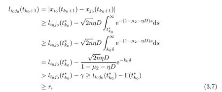

Obviously,the inequalities (3.7) and (3.8) contradict the fact that there exists (i0,j0) such thatli0j0(tk0+1)=r.Thustk0+1=∞.
Ifn0>1,with arguments similar to those in the proof of Theorem 3.1,by using the fact that

we claim thattk0+1=∞too.
Noticing that

is bounded uniformly ont,we see that the limit

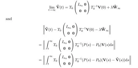
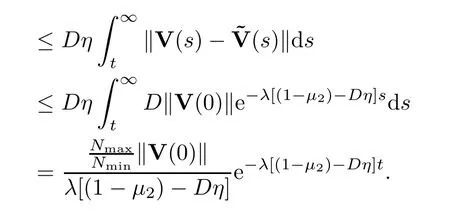
Using the triangle inequality,we have that
With arguments similar to those in the proof of Theorem 3.1 and associated discussions,we conclude that the system achieves a flock whenn0=1,and achieves a flock or multi-cluster whenn0>1.This completes the proof. □
4 Dynamics Analysis for the Delayed Model
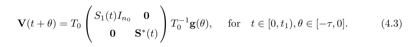
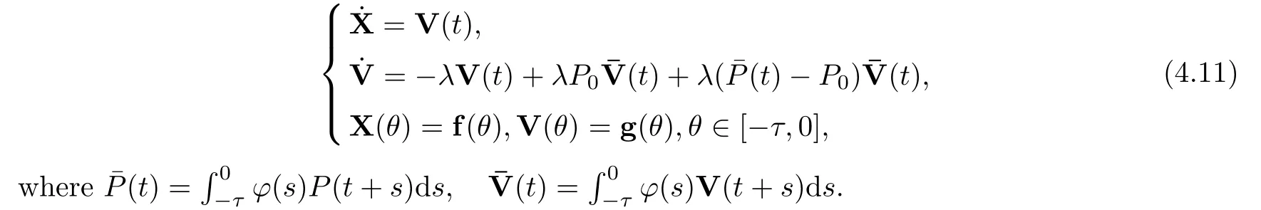
In this section,we investigate the effects of the distributed communication delay to the dynamics of system (1.1)–(2.1).Also,assume that the average matrixP(θ) remains unchanged in initial time;that is,P(θ) ≡P0forθ∈[-τ,0].Then we rewrite system (1.1)–(2.1) in a vector form,as

LetS1(t) be a fundamental solution of the equationdsand let S*(t) be a fundamental solution of the equation
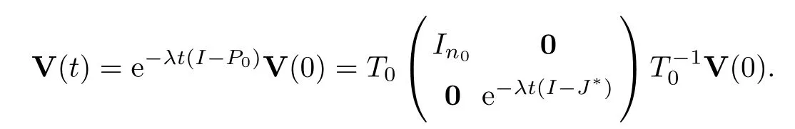
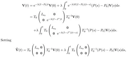
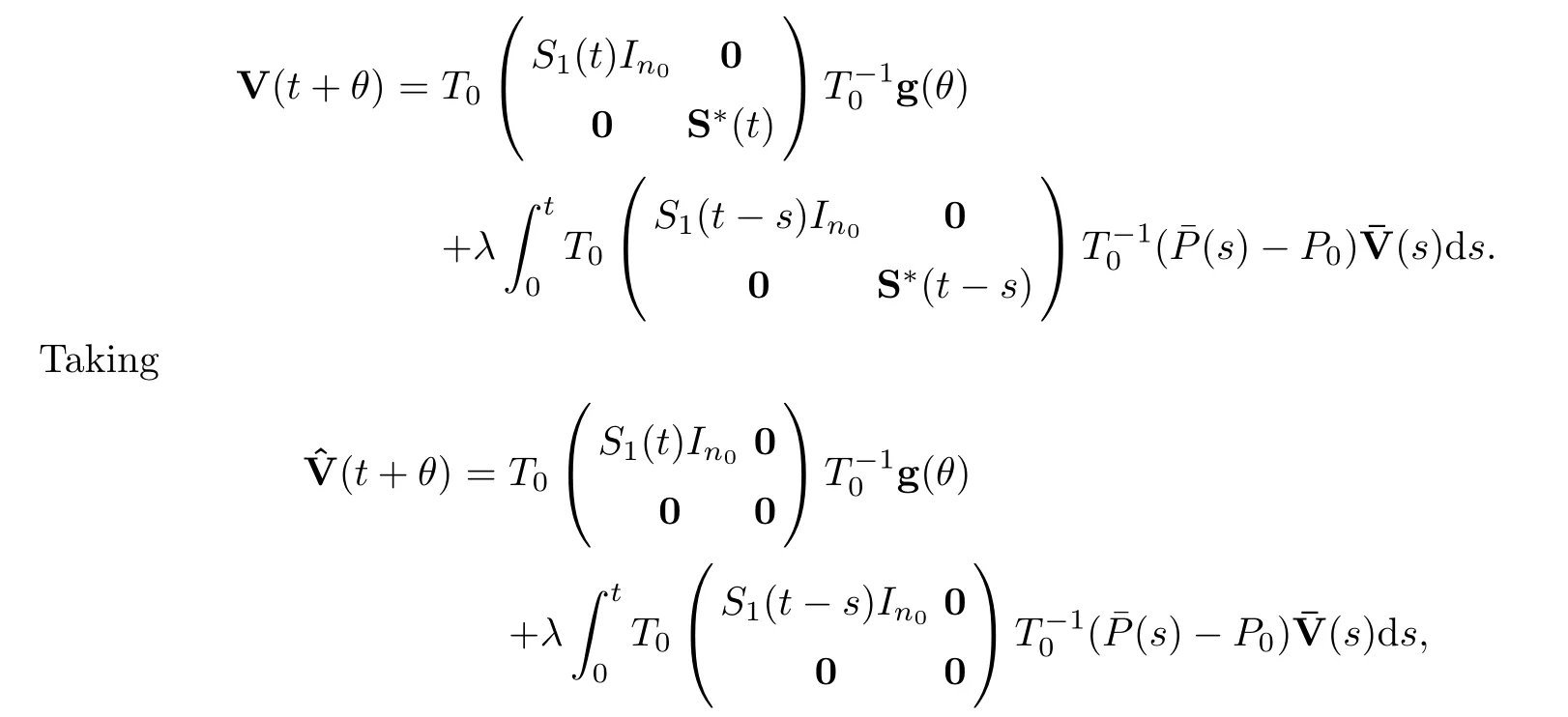
Then the solutionV(t) of (4.1) is
The characteristic equation of the first part in (4.2) is an algebraic equation

and the characteristic equation of the second part in (4.2) is
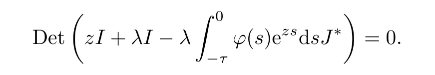
AsJ*is a Jordan block matrix,the above equation becomes

wherem0is the number of the different eigenvalues ofP0,andpiis the corresponding algebraic multiplicity.To find the convergence rate,we establish the following lemma (the details of the proof can be found in Appendix B):
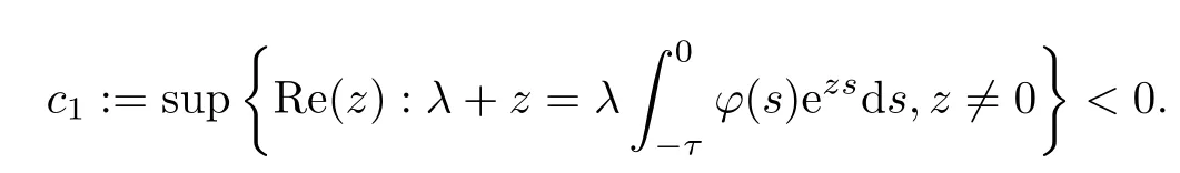
Lemma 4.1Letλ >0 and.Ifλ+1>0,then equation (4.4) has a simple root at zero and all other roots have negative real parts,and
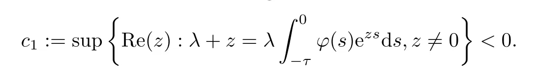
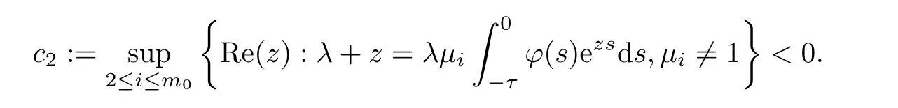
Ifμi∈(-1,1),then all roots of (4.5) have negative real parts and
Lemma 4.2([10],Theorem 5.2) Ifa0=max{Rez:h(z)=0},then,for anyα >a0,there is a constantK=K(α) such that the fundamental solutionX(t) of the second equation(4.2) satisfies the inequality

wherec0=min{|c1|,|c2|},.In particular,whenn0=1,the system achieves a flock.Whenn0>1,the system achieves a flock or multi-cluster.
First,to find the convergent rate,we decompose the solution operatorS1(t) in null-subspace.It follows from the theory of functional differential equations [10] that the spaceC([-τ,0],R)can be decomposed by the invariant null-subspaceC0and its complement.From Lemma 4.1,and the fact that the zero eigenvalue is simple,we see thatC0is a one-dimensional space.ThusS1(t)=a0+bt,wherea0∈C0is a constant operator.
Letting
we have following technical lemmas:
Lemma 4.4Let (A1) andλ||<1 hold.Then there is a positive constantKsuch that

ProofRecalling the equalities (4.3) and (4.6),we have that
Following Lemma 4.1,we see that all other roots of the characteristic equation (4.4) have negative real parts except zero.Also,from Lemma 4.2,there is a constantK1>0 such that

for allα1∈(0,-c1),c1given in Lemma 4.1.
Similarly,notice thatS*(t) is the fundamental solution operator and all roots of the characteristic equation (4.5) have negative real parts,and from Lemma 4.2,we see that there is a constantK2>0 such that

for allα2∈(0,-c2),c2given in Lemma 4.1.

whereK=Dmax{K1,K2} andc=min{α1,α2} ∈(0,c0).Thus,

This completes the proof. □
Lemma 4.5If<c0Γ(0),thent1=∞andP(t) ≡P0for all time.
ProofIft1<∞,then the average matrix will change att=t1.Thus there exists (i0,j0)such that

Recalling the first equation of (1.1),we have thati0(t)=vi0(t) and that

Ifn0=1,then all the row components ofVin(θ) are the same.From Lemma 4.3,we get that

Whenθ∈[-τ,0] andj0Ni0(0),we have that
This implies that

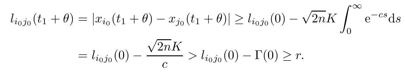
Similarly,whenθ∈[-τ,0] andj0∈Ni0(0),we have that
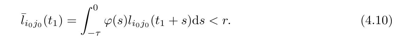
Obviously,the inequalities (4.9) and (4.10) contradict the fact that there exists (i0,j0) such thatThust1=∞andP(t) ≡P0for all time.
Ifn0>1,with arguments similar to those in the proof of Theorem 3.1,we conclude thatt1=∞.This completes the proof. □
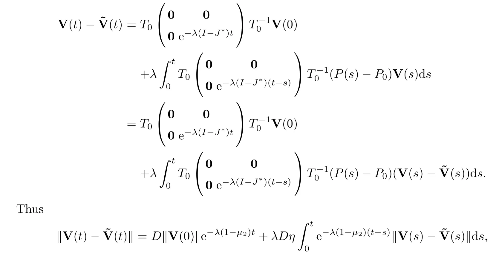
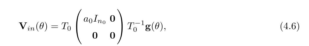
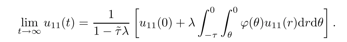
Proof of Theorem 4.3For the non-critical neighbourhood situation case,it follows fromthat the average matrix remains unchanged,and the initial matrixP0is a constant matrix for allt >0.In order to formulateVin(θ),let (u1(t),u2(t),···,un0(t),u*(t))Tbe a solution of system (4.2),and from Lemma 4.1 directly,we see that.Denoteu11(t) as the first component ofu1(t).First,we calculate the limit ofu11(t) ast→∞.Using a similar argument as for that in [1,21],consider the initial functional spaceC([-τ,0],R),which is the Banach space of real-valued continuous functions on [-τ,0] equipped with the supremum norm.LetC*=C([-τ,0],R),and define the bilinear form 〈ψ,φ〉cforφ∈Candψ∈C*by
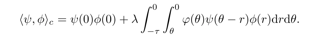
Since the characteristic equation (4.4) has a simple root at zero,its characteristic subspace is a one-dimensional space,say,C0.Denote bythe dual one-dimensional space.Let the constant functionφ(θ)=1 be the basis ofC0.Then its dual basis inwith〈ψ,φ〉c=1,where
Also,letat(θ)=u11(t+θ) for allθ∈[-τ,0].It follows from the theory of Functional Differential Equations [10] that the spaceCcan be decomposed using the invariant subspaceC0and its complement.Thusat=+bt,where∈C0.Following Lemma 4.1,we see that the characteristic equation has a simple root at zero and all other roots have negative real parts.Thusuniformly forθ∈[-τ,0].Noting thatis a constant and is determined by the initial condition,we conclude that it is given as the constant functionThus,by direct calculation,we have that
Similarly,fori=2,···,n,we obtain that
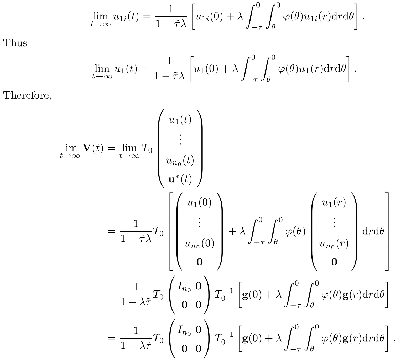
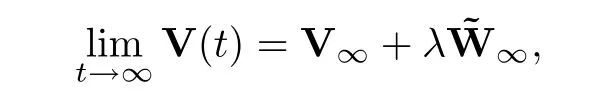
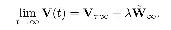
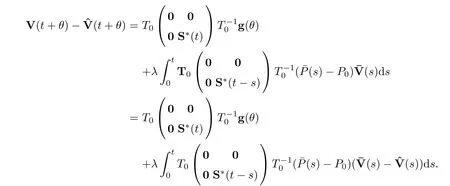
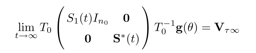
Also,from Lemma 4.4,we see tha.This means that Vin(θ) is independent ofθand that

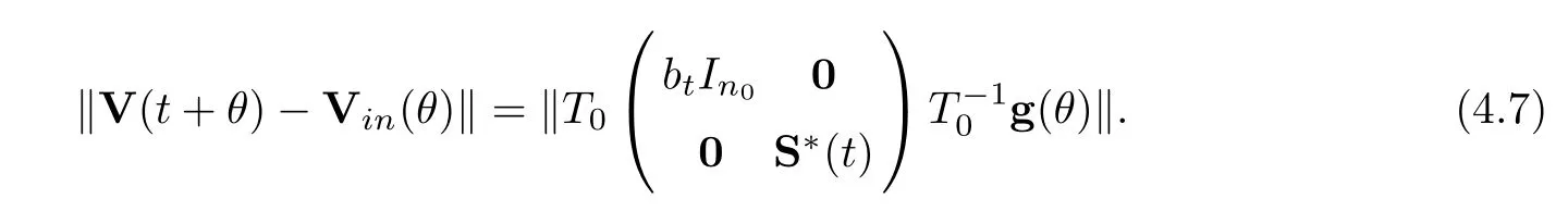
Using Lemma 4.4 again,we see that

As mentioned in (3.5),whenn0=1,all the row components of Vτ∞are the same.Furthermore,we have that


Thus system (1.1) achieves a flock asn0=1.Also,it follows from Theorem 3.1 that system(1.1) achieves a flock or multi-cluster whenn0>1.This completes the proof. □
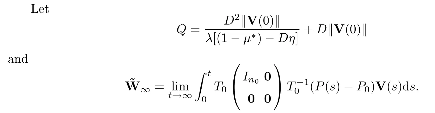
Letting

for general situation case,we have the following result:
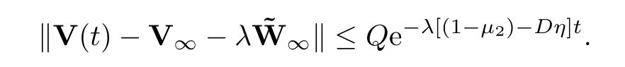
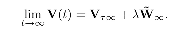
Theorem 4.6Assume that (A1),(A2τ) and (A3) hold.IfληDK2<|c2|,then
whereK2andc2are given in (4.8) and Lemma 4.1,respectively.In particular,whenn0=1,the system achieves a flock.Whenn0>1,the system achieves a flock or multi-cluster.
ProofTo investigate the flocking behaviors of system (1.1) in the general situation,we rewrite it as

we have that
It follows fromληDK2<|c2| and (4.8) that there is ac∈(0,|c2|) such thatληDK2<cand‖S*(t)‖ ≤K2e-ct.Noting that
we have that
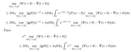
By solving the above Gronwall’s inequality,we get that

Recalling the inequalityληDK2<c,we find that there is a positive integer numberk1such that
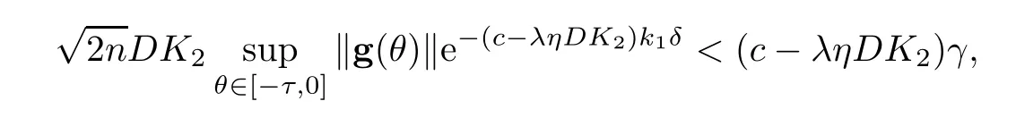
whereδandγare given as in Assumption (A2τ).
Next,we show thattk1+1=∞.Indeed,iftk1+1<∞,then there exists (i0,j0) such that
Ifn0=1,for allθ∈[-τ,0] and,we have that

This implies that
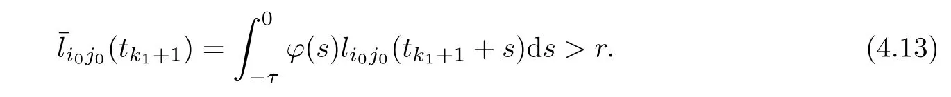
Also,for allθ∈[-τ,0] and,we have that
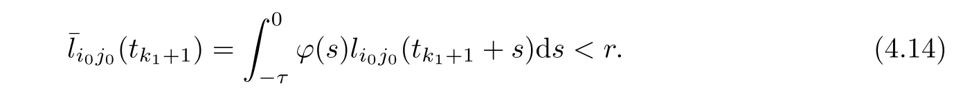
Obviously,the inequalities (4.13) and (4.14) contradicts the fact that there exists (i0,j0) such thatThustk1+1=∞andP(t) ≡Pk1for all timet >tk1.Ifn0>1,with arguments similar to those used in the proof of Theorem 3.1,we conclude thattk1+1=∞.
Using Theorem 4.3,we have that
uniformly forθ∈[-τ,0].Also,for the solution operator ‖S1(t-s)‖ being bounded,sayM0,we see that
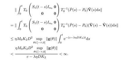
Then the limit
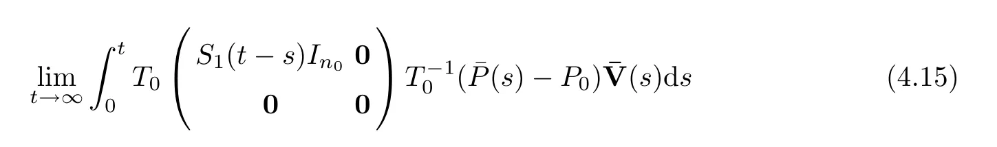

Combining this with the inequality (4.12),we have that
With arguments similar to those in the proof of Theorem 3.1 and associated discussions,we conclude that the system achieves a flock whenn0=1,and achieves a flock or multi-cluster whenn0>1.This completes the proof. □
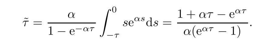
Remark 4.7Finally,we consider two kinds of particular cases: those of uniform distribution and those of exponential distribution.For the normal uniform distribution on [-τ,0],In this case,For the normal exponential distribution on[-τ,0],.Then
Appendix A
Lemma A.1If 1 is a semi-simple eigenvalue of the stochastic matrixP0with multiplicityn0,thenP0is a block diagonal matrix (if necessary,we exchange the rows of matrixP0and renumber the subscript).
Proof(for more details refer to [20]) Without loss of generality,we assume that the zeroone vectorsa1,···,an0are of the following forms (if necessary,we exchange the rows of matrixP0and relabel the subscript ofvi):
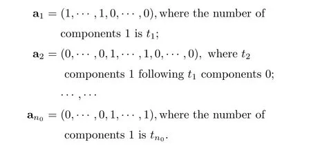
Also,we see thattiis the minimum number of components 1 inaiand thatt1+t2+···+tn0=N.In this case,noting thatP0ai=ai(i=1,···,n0) and thatpij≥0,we see thatP0is a block diagonal matrix;that is,

This completes the proof.□
Appendix B
Proof of Lemma 4.1Letdsfor givenμi∈(-1,1].We first claim that iff(z)=0 has a rootzwith Re(z) ≥0,thenzmust be zero andμi=1.In fact,if we letz=x+iywith the real partx≥0,then
Now the above inequality is strict wheneverx >0 ory≠0 orμi<1.Thus,f(z)=0 holds forx=y=0 andμi=1,which proves the claim.Therefore,all roots off(z)=0 have negative real parts,except possibly for a root at zero.Furthermore,it follows fromf′(0)=1 +λ>0 that zero is a simple root whenμi=1.Thus,the equation (4.4) has a simple root at zero and all other roots have negative real parts when 1 +λ>0,and all roots of (4.5) have negative real parts.

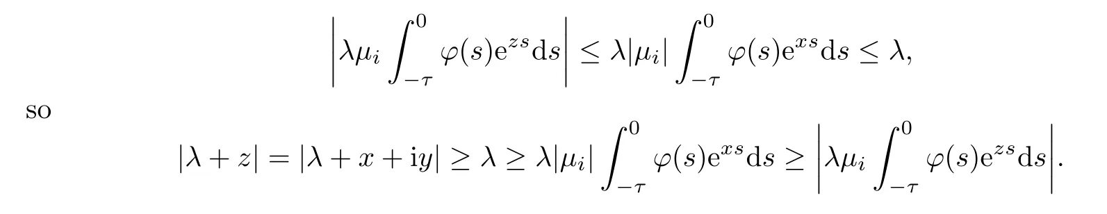
Ifc1=0,then there is a sequence {zn} (zn=xn+iyn≠0) with
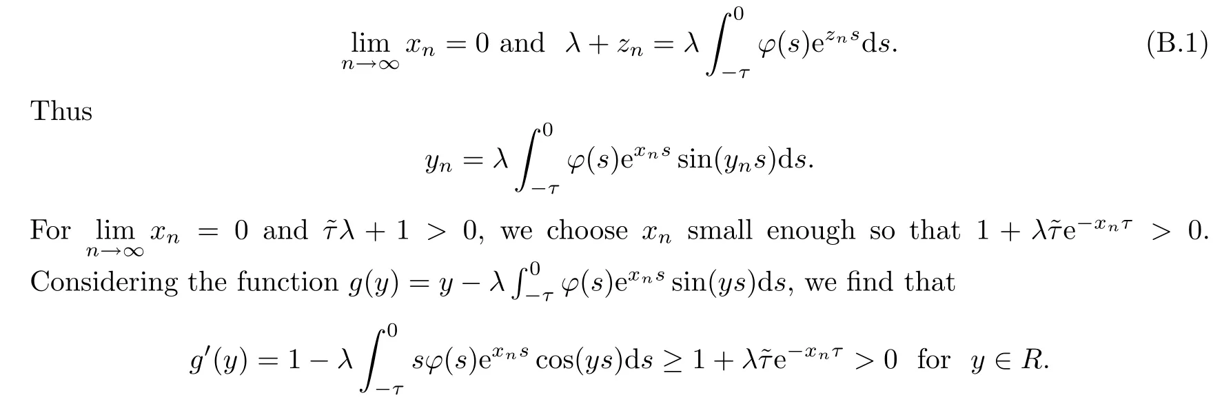
Thusy=0 is the unique root of equationg(y)=0 onRwhenxnis small enough.This contradicts (B.1).Thus
Similarly,ifc2=0,then there is a sequence {zn} with

Lettingn→∞,we have thatλ|μi| ≥λ,which contradicts the fact thatμi∈(-1,1).Thusc2<0.This completes the proof.
 Acta Mathematica Scientia(English Series)2022年5期
- Acta Mathematica Scientia(English Series)的其它文章
- ERRATUM TO: SEEMINGLY INJECTIVE VON NEUMANN ALGEBRAS(Acta Mathematica Scientia,2021,41B(6): 2055–2085.)*
- THE ASYMPTOTIC BEHAVIOR AND SYMMETRY OF POSITIVE SOLUTIONS TO p-LAPLACIAN EQUATIONS IN A HALF-SPACE*
- GLOBAL WELL-POSEDNESS FOR THE FULL COMPRESSIBLE NAVIER-STOKES EQUATIONS*
- POINTWISE SPACE-TIME BEHAVIOR OF A COMPRESSIBLE NAVIER-STOKES-KORTEWEG SYSTEM IN DIMENSION THREE*
- PROBING A STOCHASTIC EPIDEMIC HEPATITIS C VIRUS MODEL WITH A CHRONICALLY INFECTED TREATED POPULATION*
- GLOBAL STRUCTURE OF A NODAL SOLUTIONS SET OF MEAN CURVATURE EQUATION IN STATIC SPACETIME*