
H¨OLDER CONTINUOUS SOLUTIONS OF BOUSSINESQ EQUATIONS?
2018-11-22 09:24:06TaoTAO陶濤
Tao TAO(陶濤)
School of Mathematics Sciences,Peking University,Beijing 100871,China;School of Mathematics,Shandong University,Jinan 250100,China
E-mail:taotao@amss.ac.cn
Liqun ZHANG(張立群)
Academy of Mathematic and System Science,CAS,Beijing 100190,China;School of Mathematical Sciences,UCAS,Beijing 100049,China
E-mail:lqzhang@math.ac.cn
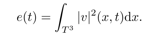
Abstract We show the existence of dissipative H?lder continuous solutions of the Boussinesq equations.More precise,for anya time interval[0,T]and any given smooth energy pro file e:[0,T] → (0,∞),there exist a weak solution(v,θ)of the 3d Boussinesq equations such thatThis extend the result of[2]about Onsager’s conjecture into Boussinesq equation and improve our previous result in[30].
Key words Boussinesq equations;H?lder continuous solutions;prescribed kinetic energy
1 Introduction
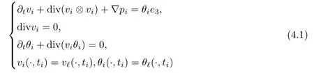
In this paper,we consider the Boussinesq equations
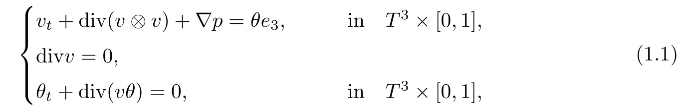
where T3denote the 3d torus,i.e.,T3=S1×S1×S1and e3=(0,0,1)T.Here in our notations,v is the velocity vector,p is the pressure,θ denotes the temperature or density which is a scalar function.The Boussinesq equations model many geophysical flows,such as atmospheric fronts and ocean circulations(see,for example,[23,25]).
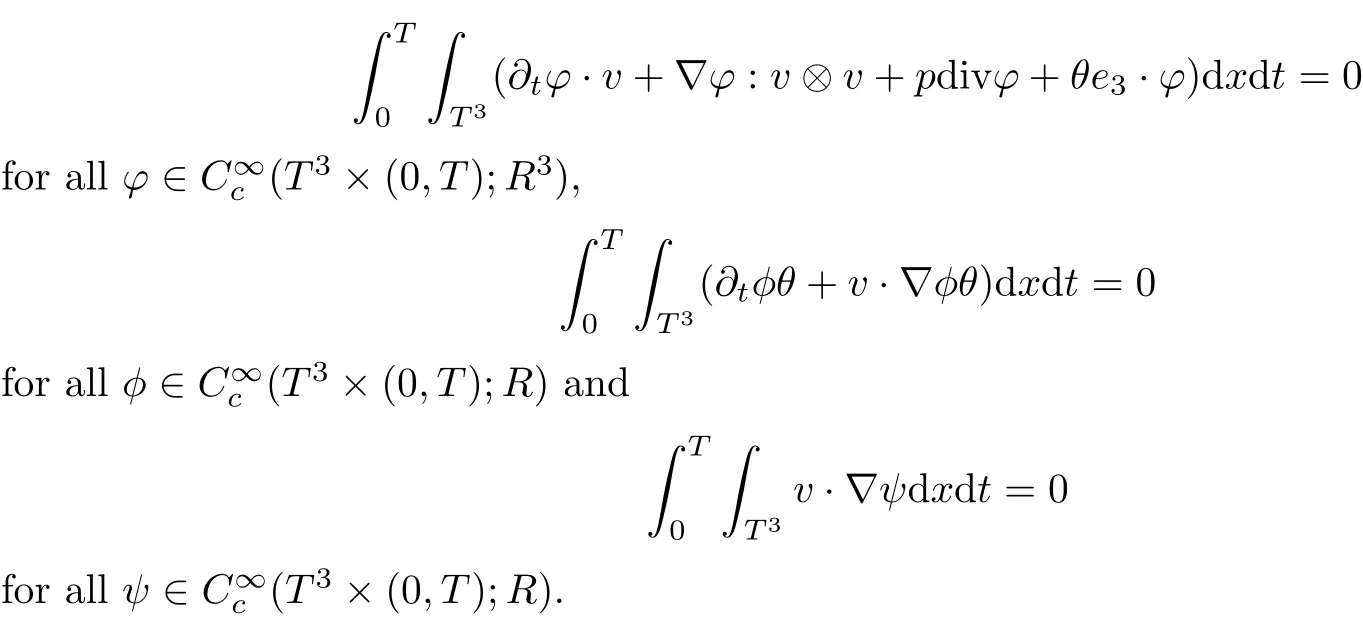
The study on weak solution of equation is important in modern theory of PDEs.The pair(v,θ)on T3× [0,T]is called a weak solution of(1.1)if they belong toand solve(1.1)in the following sense:
Moreover,consideration on weak solutions in fluid dynamics,including those which fail to conserve energy,is natural in the context of turbulent flows.One famous example is the Onsager conjecture for incompressible Euler equation which claims that this equation admits H?lder continuous dissipative solution.Precisely,Onsager conjecture for the incompressible Euler equation can be stated as follows:
(1)C0,αsolutions are energy conservative when α >.
About this conjecture,the part(a)was proved by Constantin,E and Titi in[9].Slightly weak assumption on the solution was subsequently shown to be sufficient for proving part(a)by Constantin,etc.in[6,17],also see[29].More recently,Isett and Oh gave a proof to this part for the incompressible Euler equations on manifold by heat flow method in[18].
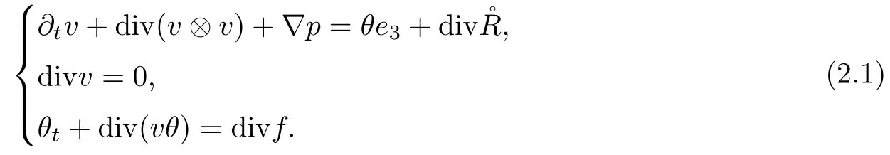
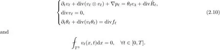
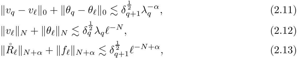
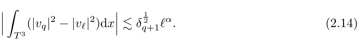
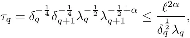
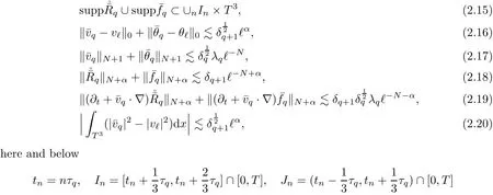
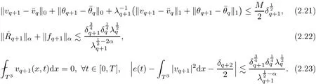
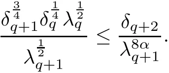
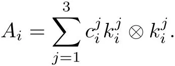
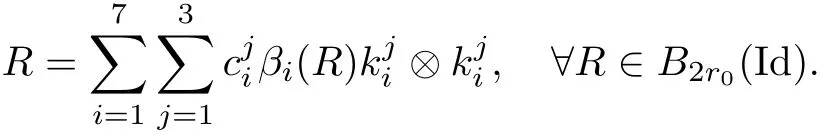
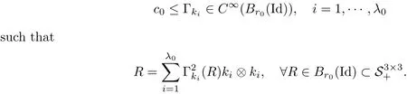
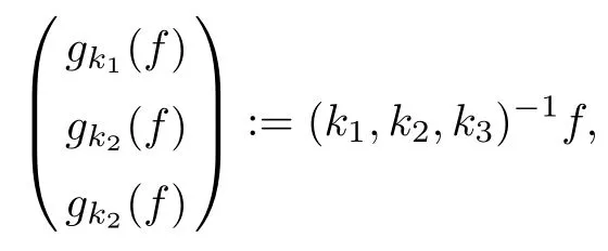
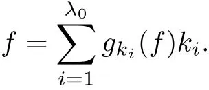
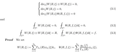
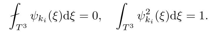
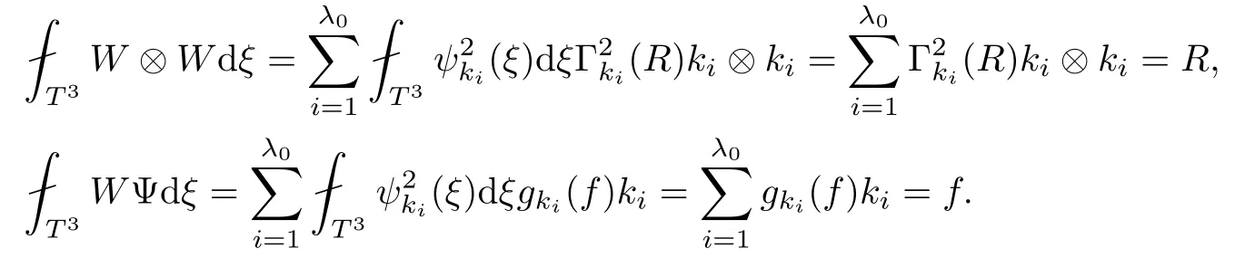
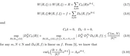
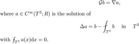
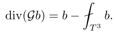
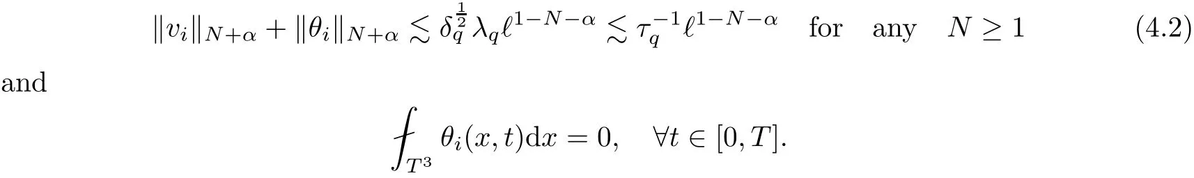
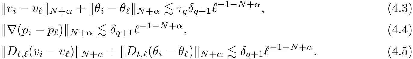
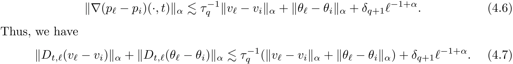
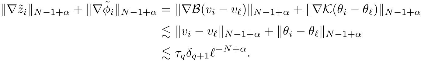
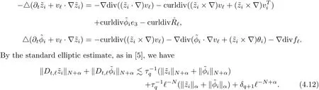
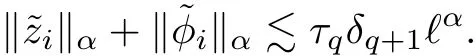
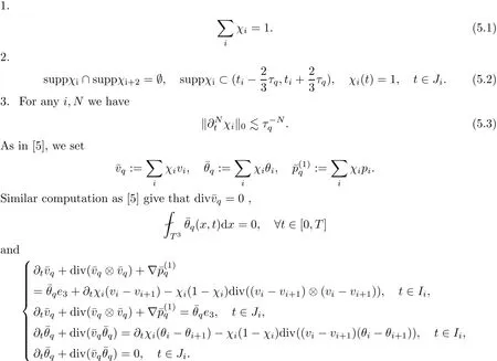
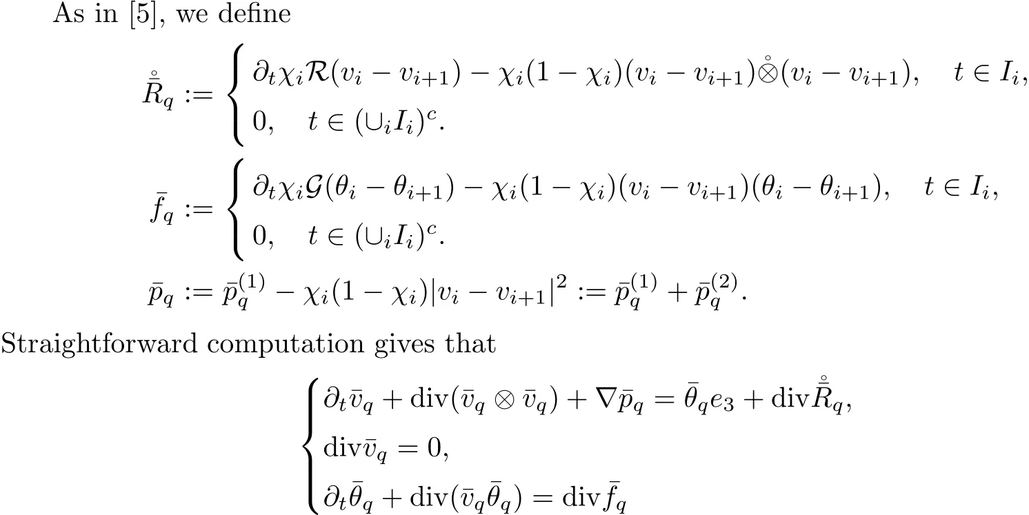
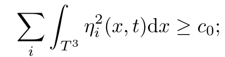
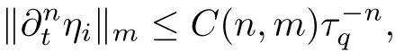
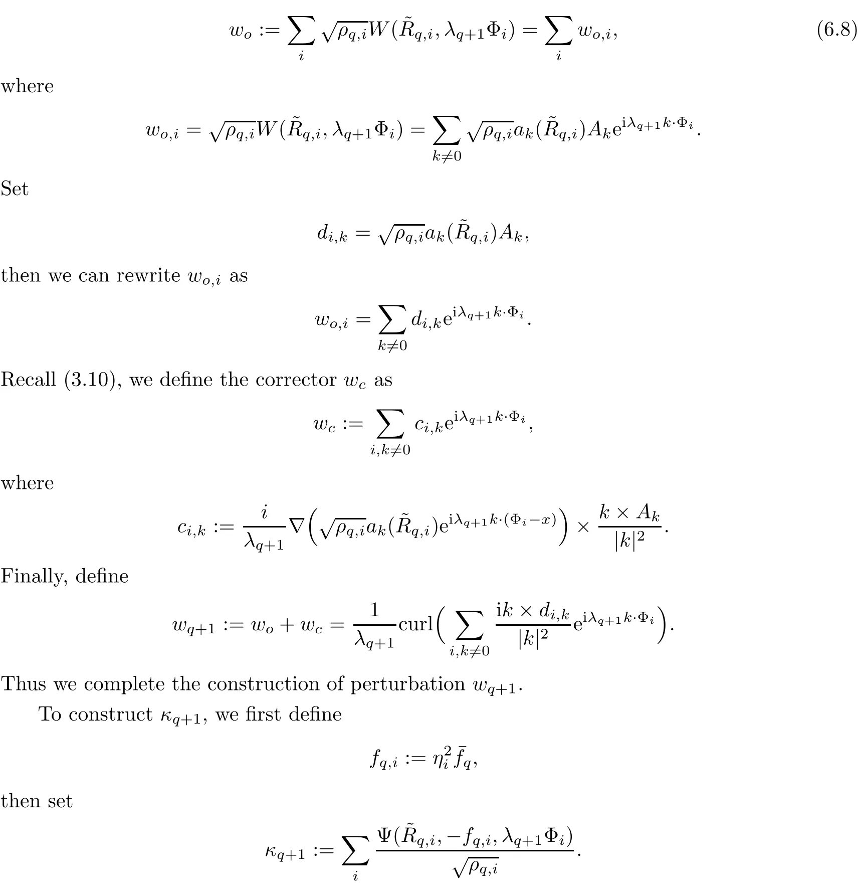
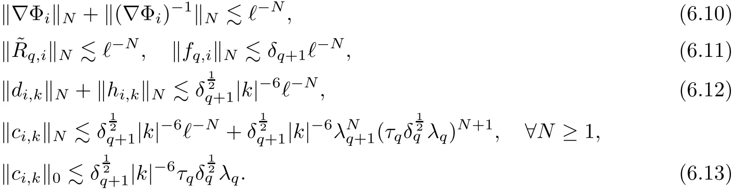
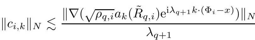
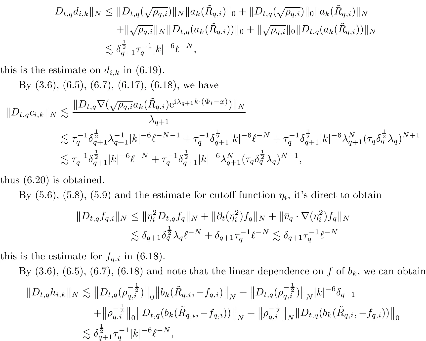
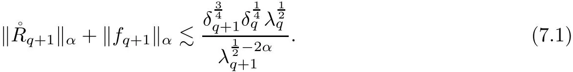
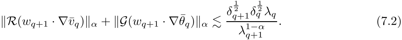
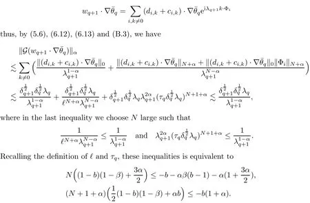
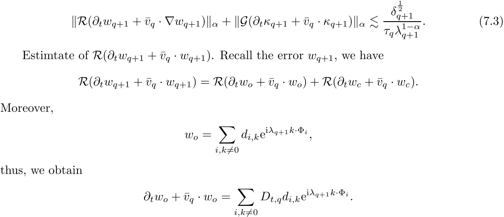
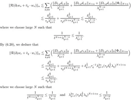
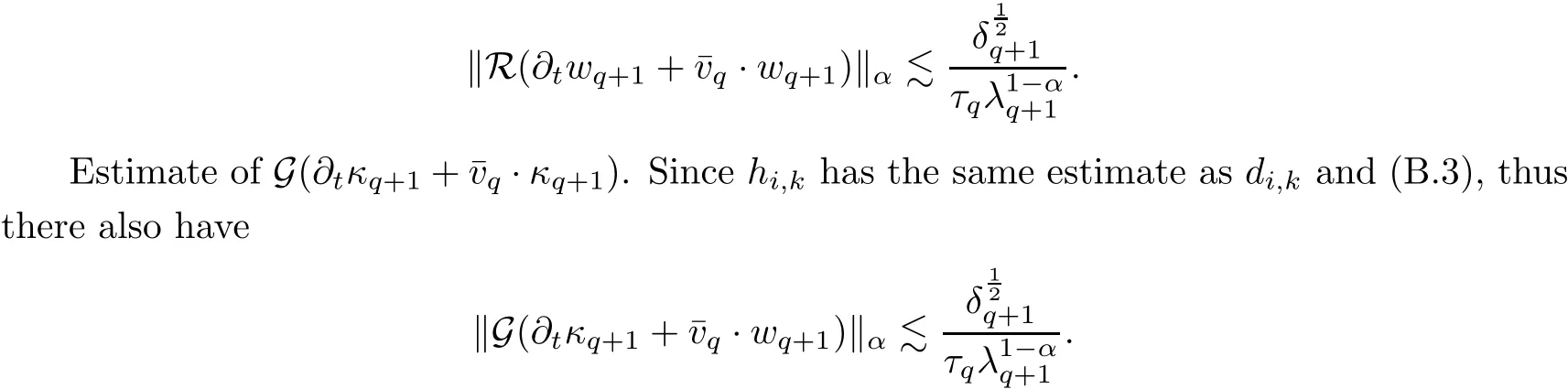
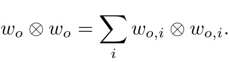
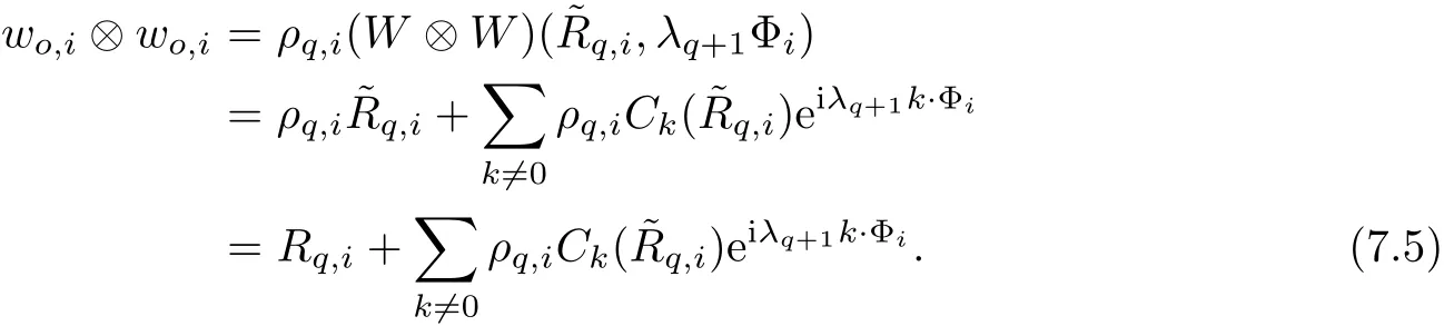
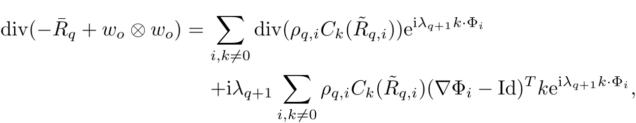
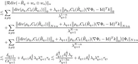
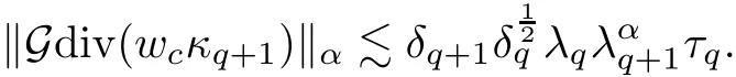
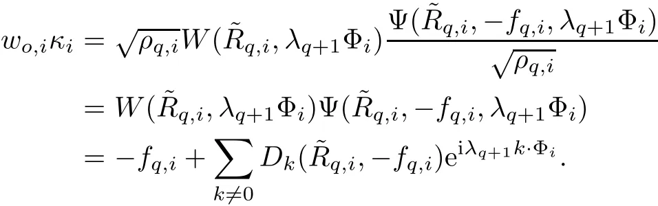
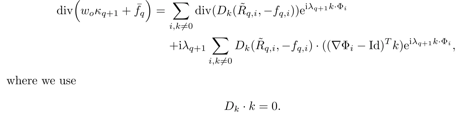
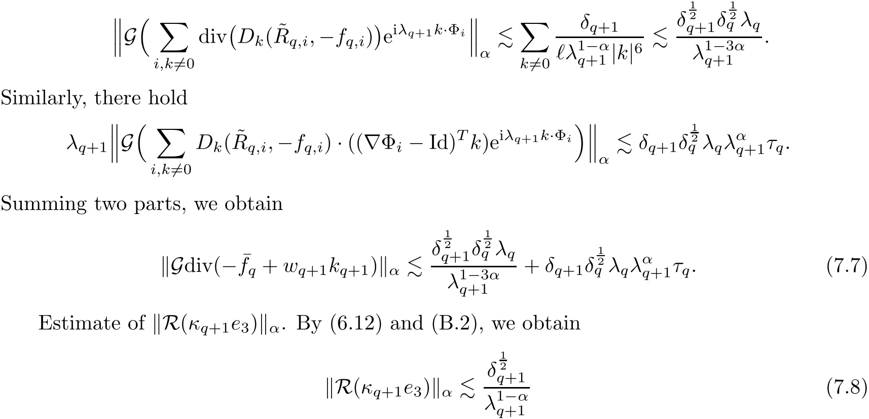
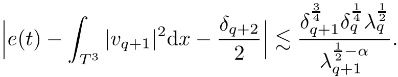
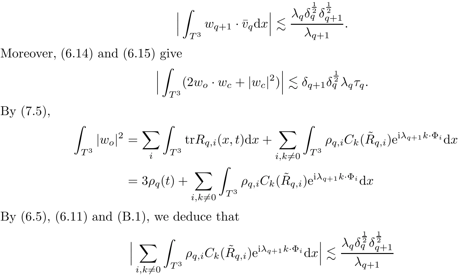
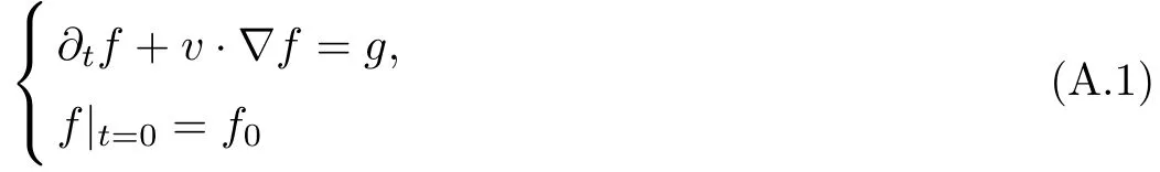
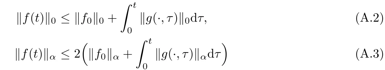
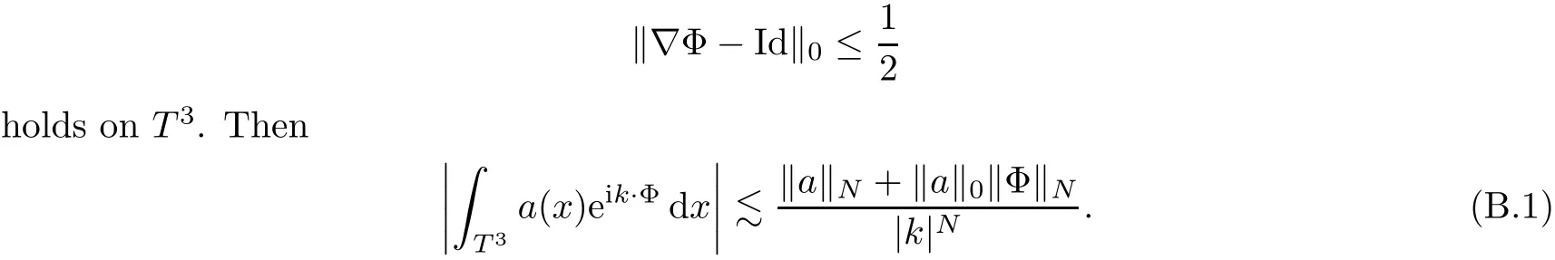
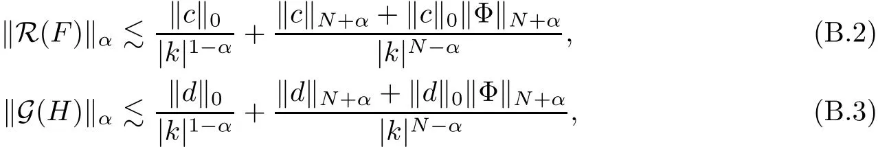
The part(b)has been treated by many authors from the nineties.For weak solutions,there are some results by Sche ff er(see[26]),Shnirelman(see[27,28])and De Lellis,Sz′ekelyhidi(see[12,13]).A great progress in the construction of H?lder continuous solution was made by De Lellis,Sz′ekelyhidi,Isett and Buckmaster in recent years.The key breakthrough was made by De Lellis and Sz′ekelyhidi in[15]where they developed an iterative scheme(some kind of convex integration).With the help of Beltrami flow on T3and geometric lemma,they constructed a continuous periodic solution which satis fies the prescribed kinetic energy.The solution is a superposition of in finitely many and weakly interacting Beltrami flows.Based on the iterative techniques developed in[15]and Nash-Moser mollify techniques,they constructed H?lder continuous periodic solution with exponent θ,for any θ<,which satis fies the prescribed kinetic energy in[16].Later,Isett introduced some ideas and constructed H?lder continuous periodic solutions with any θ For the Onsager critical spatial regularity(H?lder exponent θ=),there are also some important results.In line with previous iterative scheme,by keeping track of sharper,time localized estimates,Buckmaster in[1]constructed H?lder continuous(with exponent θ Motivated by Onsager’s conjecture for Euler equation,we study Boussinesq equations and want to know if anomalous dissipation phenomena still happen when considering the temperature e ff ects.The di ff erence is that there are conversions between internal energy and mechanical energy.What we need is to overcome the difficulty of interactions between velocity and temperature.Here,following the general scheme of the construction of Euler equations in[5]and by establishing the corresponding geometric lemma and constructing a special stationary solution of Boussinesq equation(we call it generalized Mikado flow),we obtain the similar result as[2]and improve the regularity of solution in our previous work[30]. Theorem 1.1Assume that e(t):[0,T]→R is a given positive smooth function and ε∈(0,).Then there exist such that they solve the system(1.1)in the sense of distribution and Remark 1.2In our Theorem 1.1,if θ=0,then it’s the H?lder continuous Euler flow with prescribed kinetic energy and have been constructed in[2].In general,we can construct nonzero θ by choosing the initial nonzero temperature in the iterative procedure. Remark 1.3The above theorems also hold for the two-dimensional Boussinesq equations on T2. Finally,we brie fly summarize some main ideas in our proof.Following the ideas in[5],we establish the related geometric lemma and construct a special stationary solution of Boussinesq equation(we call it generalized Mikado flow)by adding together“straight-pipe” flow supported in disjoint cylinder that point in multiple direction(the method is from[11]).Using this generalized Mikado flow in the convex integration,we can deal with the interaction of waves with di ff erent direction which is in sharp contrast to our technique in[30]where we only add wave with same direction in one step because we can’t control the interaction of wave with di ff erent direction.Thus,we use one-step iteration scheme which is key to improve the regularity of solution.Moreover,as in[5],the process of our construction also consists of three stages:molli fication,gluing and perturbation. The rest of paper is organized as follows.In Section 2,we give a proof of our theorem and describe the construction.In Sections 3,4,we gives some preliminaries.We establish the gemmetric lemma and “generalized Mikado flow”by the method of[11]and construct a new operator G which will be be used in order to deal with the stress arising from iteration scheme.After preliminaries,gluing process and perturbation step are performed,respectively,in Sections 5,6.Finally,in Section 7,we establish the estimate for stress error and close the iteration. As in[5],the proof of Theorem 1.1 will be achieved through an iteration procedure.In this and the subsequent sections,denotes the vector space of symmetric trace-free 3×3 matrices. De finition 2.1Assumeare smooth functions on T3×[0,T]taking values,respectively,in.We say that they solve the Boussinesq-Stress system if We now state the main proposition of this paper,of which Theorem 1.1 are implied directly.The proposition is also an extension of the corresponding result given in[15].As in[5],we set parameters λq,δqas following As in[5],we impose that the energy pro file satis fies Proposition 2.2There is a universal constant M such that the following properties hold: Then there exists α0depending on β,b such that for any α ∈ (0,α0),we can find a0depending on β,b,α,M such that for all a ≥ a0the following holds:given e(t)as in Theorem 1.1 and satis fies(2.2),solves(2.1)and satis fies then we can construct new functions,they also solves Boussinesq-Stress system(2.1)and satis fies(2.4)–(2.7)with q replaced by q+1.Moreover,the following hold Theorem 1.1 is obtain directly by using Proposition 2.2 inductively and the proof is similar as[5],we omit the detail here. Next,we outline the proof of Proposition 2.2 and it also consists of three stages as in[5]. As in[5],we make assumption on parameter:α is sufficiently small such that and our proof also consists of three stages: As in[5],take ψ be a standard molli fication kernel,set by choosing α sufficiently small and a sufficiently large.Then,de fine A straightforward computation gives that As in[5],we also have the following estimates and the proof is same as[5],we omit it here. Proposition 2.3For any N≥0, As in[5],we introduce another parameter and the implicit constants depend only on M,N,α. As in[5],we construct new solutionby adding generalized Mikado flow and obtain the following estimates This step will be given in Sections 6 and 7. By combining the estimate(2.11)–(2.14),(2.16)–(2.23)and choosing suitable parameter a,b,this proposition can be proved by the similar method in[5].In fact,to close the iteration, we only need to choose α,a,b such that Recall the form of δq,λq,the above inequality is equivalent to This is equivalent to We introduce some notations:R3×3denotes the space of 3×3 matrices;denotes the spaces of 3×3 positive de finite symmetric matrices and Id denotes 3×3 identity matrix.The matrix norm The following lemma is an extension of geometric lemma given in[11]to our case.Within it,we not only represent a prescribed symmetric matrix R infor some r0>0,but also a prescribed vector simultaneously. Lemma 3.1(geometric lemma) There exist constant r0>0,c0>0,λ0≥ 1 and positive smooth functions and linear functions such that ProofThe proof of(1)is based on convex analysis.Choosing 7 positive de finite symmetric matrix A1,···,A7such that Id belong to the interior of their convex hull in,which is a open convex simplex S.We choose r0>0 such that the ballis contained in S. and the functions βiare positive and smooth on Moreover,for every positive de finite matrix Ai,there exist three vectorsand positive constantsuch that Thus,we obtain Thus,the proof of the first part of this lemma is complete. Next,we give a proof on the existence of gkand the related property.Let us assume that vectors(k1,k2,k3)are linear independent,and set gki(f)=0 for k 6=ki,i=1,2,3 and Then we finished the proof of the geometric lemma. The following lemma is an extension of Mikado from in[11]. Lemma 3.2Forwhere r0is from Lemma 3.1,there exist smooth functions such that for everythe following property holds where λ0,ki,Γki,gkiare from Lemma 3.1,and ψki(ξ)=hki(dist(ξ,lki,pki))with hki∈C∞c([0,rki)),rki>0,where lki,pkiis the T3-periodic extension of the line{pki+tki:t∈R}passing though pkiin direction ki.Since there are only a finite number of such lines,we may choose pkiand rkiin such a way that Thus W consistes of a finite collection of disjoint straight tubes such that in each tube W is a traight pope flow and outside the tubes W=0.In particular,a straightforward computation give(3.1). Furthermore,the pro file functions hkiwill be chosen so that for all ki Thus it’s easy to get(3.2).Using(3.4)and Geometric Lemma 3.1 we also have Therefore,(3.3)is satis fied.The proof of Lemma 3.2 is completed. Using the fact that W(R,ξ),Ψ(R,f,ξ)is T3-periodic and has zero mean in ξ,we write for some coefficients ak(R),bk(R,f)and complex vectorsatisfying Ak·k=0 andMoreover,bk(R,f)is linear about f.From the smoothness ofandwe further infer Using the Fourier representation in above,we see that from(3.3) We introduce two operators in order to deal with the Reynold stresses.The operator R was introduced in[15]and the operator G is given by us. 3.3.1 The Operator R The following lemma is taken from[15],we copy it here for the completeness of the paper(the proof can be found in[15]). Lemma 3.3(R=div?1) There exist a linear operator R from C∞(T3,R3)to C∞(T3,R3×3)such that the following property hold:for any v∈C∞(T3,R3)we have (a)Rv(x)is a symmetric trace-free matrix for each x∈T3; 3.3.2 The Operator G De finition 3.4Let b∈ C∞(T3;R)be a smooth function.We de fine a vector-valued periodic function Gb by Lemma 3.5(G=div?1)For any b∈C∞(T3;R),we have ProofThe proof is elementary.In fact,we calculate directly Some estimates related to the operators R and G can be founded in the Appendix A.2. For each i,let ti=iτq,and consider smooth solutions of the Boussinesq equations de fined over their own maximal interval of existence. As in[5],we have the following estimates:If a is sufficiently large and|t?ti|≤ τq,we have For convenience,as in[5],we de fine Dt,?= ?t+v?·? to be the material derivative associated with v?.Similar to[5],we also have the following stability estimate. Proposition 4.1For,there hold ProofWe first consider(4.3)with N=0.From(2.10)and(4.1),we have As in[5],by elliptic estimate for pressure,we obtain By the transport estimate as in[5](also see(A.3)),we obtain Gr?nwall’s inequality give this is(4.3)with N=0.(4.4)and(4.5)with N=0 can be obtained by putting(4.3)into(4.6)and(4.7). For N≥1,the proof is similar as[5],we omit the detail. Next,as in[5],we de fine the vector potential to the solution(vi,θi)as where B is the Biot-Savart operator. Proposition 4.2For,we have that ProofThe proof is similar as in[5].Set,then Hence it sufficient to estimate For N ≥ 1,by(4.3)and the boundness of operators?B,?K on H?lder space,we have Next,we consider the case N=0.Recall Taking curl for the first equation and?for the second equation of(4.11)and using the identity curlcurl=?△+?div and(4.10),we arrive at Setting N=0,by combining transport estimate and Gr?nwall’s inequality,we arrive at Putting this estimate into(4.12)and using Gr?nwall inequality,we obtain Thus,the proof of(4.8)is completed.(4.9)follows(4.12)and(4.8). Let{Ii,Ji}ibe as above,they decompose[0,T]into pairwise disjoints intervals.The following partition of unity is standard and can be found also in[5]:there exists a partition of unity χiin time such that As in[5],we can obtain the following estimates. Proposition 5.1For all N≥0,there have The proposition can be obtained from Proposition 4.1 and the relationship of parameters?,τqby the similar argument as in[5],we omit the proof. As in[5],we also have the following estimates: Proposition 5.2For all N≥0,there have ProofThe estimate oncan be directly found in[5]and we only consider the estimates on fq.Recall that θi=divφi,we write for t∈ Ii: Thus,by(4.3)and(4.8)and note that Gdiv is a bounded operator on H?lder space,we have Finally,collecting the obtained result in this section,we obtain(2.15)–(2.20)and the gluing process is completed. For convenience,we write the following squiggling stripes,whose proof can be found in[5].There exist smooth nonnegative cut-o fffunction ηi= ηi(x,t)with the following properties: (5)There exists a positive geometric constant c0such that for any t∈[0,T] (6)For any i and n,m≥0, where C(n,m)are geometric constant depending only on n,m. First,as in[5],to de fine the amplitude of the perturbation,we de fine Lemma 6.11.We have 2.For any N≥0, 3.For a?1, First,the main perturbation on velocity can be de fined as First,set We summarize the main estimates of di,k,ci,kand hi,k. Proposition 6.2For t∈ ProofThe estimate oncan be obtained as[5],we omit it.From the de finition of ci,k,and by(3.6),(6.2),(6.5),(6.10),(6.11),we have this is the estimate for hi,kin(6.12).The proof of Proposition 6.2 is completed. From the de finition wo,wc,κq+1and the above proposition,we can obtain the following corollary: Corollary 6.3There exist a universal constant M such that if a is sufficiently large,then ProofThe proof of(6.14)is same as[5]and we omit it.The de finition of wcand(6.13)gives Thus,(6.15)is obtained.Summing the estimates on w0,wcand taking a large enough,we get the estimate on wq+1of(6.16). Similarly,by(6.12),we deduce the estimate on κq+1of(6.16).The proof of Corollary 6.3 is completed. Proposition 6.4For t∈and any N≥0,we have ProofFirst,the estimates onis similar to[5],and we only consider the estimates on By(3.6),(6.5),(6.7),estimate onin(6.18),we have this is the estimate for hi,kin(6.19).The proof of Proposition 6.4 is completed. Finally,(2.21)follows from the construction(6.9)and estimate(6.16). In this section,we prove the inductive estimates on Proposition 7.1For small α,the stress errorsatis fies the estimate As in[5],we have:for small α∈(0,1), As in[5],we have:for small α∈(0,1), By(B.2)and(6.19),we deduce that as the above subsection.Finally,summing two parts,we arrive at Collecting these estimate together,we arrive at(7.3). For small α∈(0,1),we have First,combining(6.14)and(6.15),it’s straight to obtain Then,due to the supports of the cuto ff s ηjbeing mutually disjoint,we have Using the de finition of wo,iand(3.7),we deduce that Thus,we obtain where we used the fact Ckk=0.Thus,by(6.5),(6.11),(6.2)and support property of ηi,we deduce that where we used(3.9)and as in the previous section,we choose large N.Collecting the two parts,we arrive at First,(6.15)and(6.16)give Then,using the de finition of wo,i,κiand(3.8),we deduce that Consequently,due to the supports of the cuto ff s ηjbeing mutually disjoint,we deduce that By(B.3),(3.9),(5.8),(6.10)–(6.12)and the linear dependence of Dkon f,the same argument as above gives that by choosing N large enough. Finally,(7.4)follows from(7.6),(7.7)and(7.8). Conclusion,(7.1)follows from(7.2),(7.3)and(7.4)by combining As in[5],we know that the energy of vq+1satis fies the following estimate ProofBy de finition,we have Note that wq+1is curl form and integration by parts,using(5.6),(6.12),we obtain by taking N large in(B.1).Combining the above estimates and the de finition of ρq(t),we complete the proof. ? Finally,(7.1)and this energy estimate give(2.22)and(2.23).Combining Section 6 and Section 7,we obtain(2.21)–(2.23),and complete the perturbation step.Thus,we give a proof of Proposition 2.2. Appendix A Estimate for Transport Equation In this section we gives some well known estimates for the smooth solution of transport equation: where v=v(x,t)is a given smooth vector field.The proof can be found in[2]. Proposition A.1Assume.Then any solution of(A.1)satis fies the following estimates: for all 0<α≤1.Generally,for any N≥1 and 0≤α≤1,there hold Let Φ(t,·)be the inverse of the flux X of v staring at time t0as the identity.Under the above assumption|t?t0|kvk1≤1 we have Appendix B Stationary Phase Lemma We recall here the following facts about operator R and G,where the operator R is de fined in[15](for a proof we refer to[5]). Proposition B.1 (i)Let α∈(0,1)and N ≥1.Let a∈C∞(T3),Φ∈C∞(T3;R3)be smooth function and assume that (ii)Let k∈Z3{0}be fixed.For a smooth vector field c∈C∞(T3;R3)and a smooth scalar function d ∈ C∞(T3;R).Let F(x):=c(x)eik·Φand H(x):=d(x)eik·Φ.Then we have where the implicit constant depends on α and N,but not on k. Proof(B.1),(B.2)can be found in[11].From the de finition of G,we directly arrive at the estimate(B.3)by the same method as in[11],we omit the detail here. Appendix C Commutators Involving Singular Integrals The following estimate is from[5]and we only recall it,the proof can be found in[5]. Proposition C.1Let α ∈ (0,1)and N ≥ 0.Let TKbe a Calder′on-Zygmund operator with kernel K and b ∈ CN+1,α(T3)a vector field.Then we have for any f ∈ CN+α(T3),where the implicit constant depends on α,N,K.
2 Proof of Main Theorem and Outline of the Construction
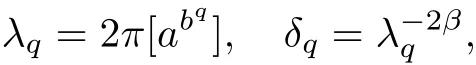
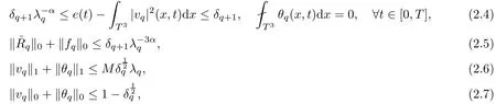
2.1 Inductive Proposition


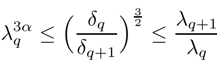
2.2 Stages
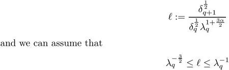
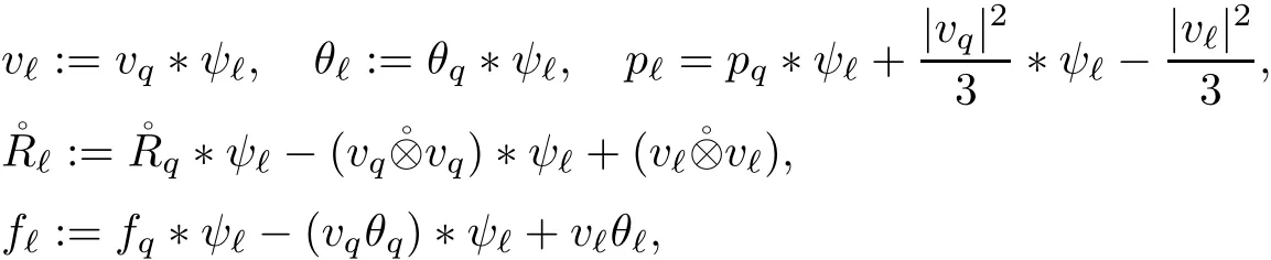
2.3 Molli fication Step
2.4 Gluing Step
2.5 Perturbation
2.6 Proof of Propositions 2.2

3 Preliminaries
3.1 Geometric Lemma


3.2 Generalized Mikado Flow


3.3 The Operator R and G

4 Stability Estimate for Classical Exact Solution


5 Gluing Procedure
5.1 Partition of Unity and De finition of
5.2 The New Stress Error
5.3 Estimate on
5.4 Estimate on Stress Error

6 Perturbation Step
6.1 The Stress Error
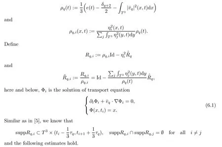


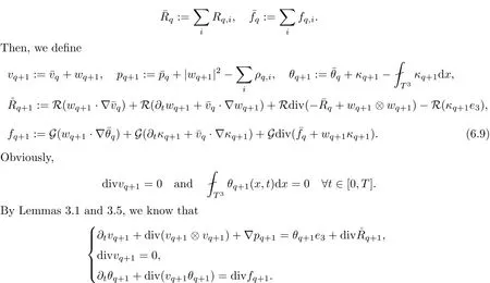
6.2 The Perturbation wq+1and κq+1
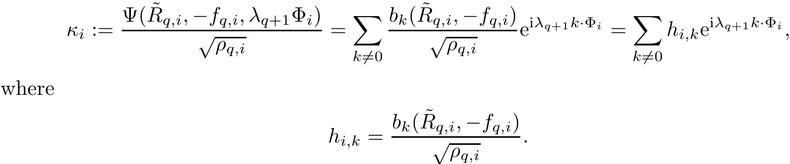
6.3 The Construction of
6.4 Estimate on the perturbation
7 Estimates on New Stress Error
7.1 Estimates on Nash Error
7.2 Estimates on Transport Error
7.3 Estimate on Oscillation Error


7.4 Energy Iterate


 Acta Mathematica Scientia(English Series)2018年5期
- Acta Mathematica Scientia(English Series)的其它文章
- REVIEW ON MATHEMATICAL ANALYSIS OF SOME TWO-PHASE FLOW MODELS?
- STRONG COMPARISON PRINCIPLES FOR SOME NONLINEAR DEGENERATE ELLIPTIC EQUATIONS?
- RADIAL SYMMETRY FOR SYSTEMS OF FRACTIONAL LAPLACIAN?
- MACROSCOPIC REGULARITY FOR THE BOLTZMANN EQUATION?
- ONE-DIMENSIONAL VISCOUS RADIATIVE GAS WITH TEMPERATURE DEPENDENT VISCOSITY?
- STABILITY OF STEADY MULTI-WAVE CONFIGURATIONS FOR THE FULL EULER EQUATIONS OF COMPRESSIBLE FLUID FLOW?