H.Wajahat A.Riaz

Department of Physics,University of Punjab,Quaid-e-Azam Campus,Lahore-54590,Pakistan

AbstractUsing a quasideterminant Darboux matrix,we compute soliton solutions of a negative order AKNS(AKNS(?1))equation.Darboux transformation(DT)is defined on the solutions to the Lax pair and the AKNS(?1)equation.By iterated DT to K-times,we obtain multisoliton solutions.It has been shown that multisoliton solutions can be expressed in terms of quasideterminants and shown to be related with the dressed solutions as obtained by dressing method.

Key words:integrable systems,solitons,Darboux transformation,quasideterminants

1 Introduction

Many integrable systems,such as Korteweg de Vries(KdV),mKdV equation admit both positive and negative hierarchy

where R is referred to as recursion operator,whereas n with the negative values correspond to negative flow of hierarchy and n with positive values are referred to as positive flow of hierarchy.A well known example of negative hierarchy is the sine-Gordon equation(which has potential applications in Josephson transmission line,[1?2]ultrashort pulse propagation in a resonant medium[3])can be derived from the mKdV equation.The coupled dispersionless integrable equations are negative flow of the non-linear Schrdinger hierarchy.Various integrable equations,such as Camnassa-Holm equation,[4?5]Degasperis-Procesi equation,[6]and the short-pulse equation[7?8]are associated to negative order equations through reciprocal transformations.The significance of the negative order equations is that one can generate infinitely many symmetries for nonisospectral Ablowitz-Ladik lattice hierarchy.[9]Note that infinitely many symmetries are usually obtained in case of isospectral hierarchies.So negative order flows provide some new interesting results not only from the point of view of integrability,but also interesting dynamically,both mathematically and physically.

Many systematic methods–inverse scattering transform(IST),Bcklund transformation,Hirota bilinear method,Darboux transformation,the trigonometric function series method,the modified mapping method and the extended mapping method,the bifurcation method etc.,have been used to compute exact solutions of various nonlinear partial differential equations in the literature(see Refs.[10]–[17]and references therein).Darboux transformation(DT)is one of the powerful and effective technique used to generate solutions of a given nonlinear integrable equation in soliton theory.Various integrable equations have been studied successfully by the approach of DT and obtained explicit solutions.Meanwhile the solutions are expressed in terms of Wronskian,quasi-Wronskian,Grammian,quasi-Grammian,and quasi-determinants in the literature.[18?24]

The present work is about to study the DT of the negative order AKNS(denoted by AKNS(?1))equation.The AKNS(?1)equation and its multi-component generalizations have been studied by virtue of Hirota method and the soliton solutions have been investigated.[25?26]Noncommutative generalization of the AKNS(?1)equation has been discussed in Ref.[27].Meanwhile,DTs and soliton solutions have also been offered.

In this paper,we study the DT of AKNS(?1)equation.We define a DT in terms of Darboux matrix on the solutions to the Lax pair and the solutions of the AKNS(?1)equation.The K-soliton solution is expressed in terms of quasideterminants.Further,quasideterminant solutions are shown to be related with the dressed solutions.We compute soliton solutions of the AKNS(?1)equation.One-,two-,and three-soliton solutions have been computed explicitly.

2 Lax Pair

We start with the Lax pair of the AKNS(?1)equation attribute to[25]

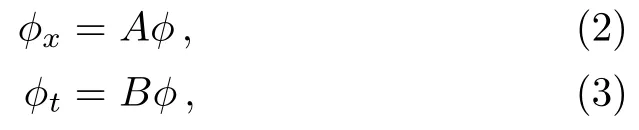
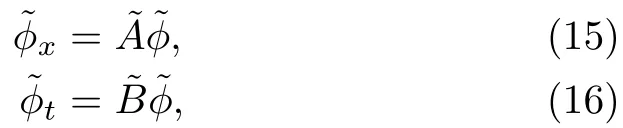
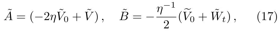
where ? = ?(x,t, η)is a 2 × 2 eigen-matrix,which depends on x,t and the spectral parameter η.The matrices A and B are given by

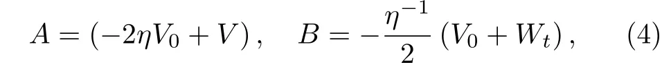
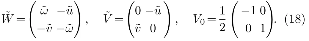
with

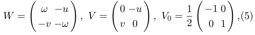
where u(x,t)and v(x,t)are scalar functions,whereas ω = ??1(uv)and ?x??1= ??1?x=1, ?x≡ ?/?x.The compatibility condition i.e.,?xt= ?txof the Lax pair(2)–(3)implies a zero-curvature condition i.e.,At? Bx+[A,B]=0,which is equivalent to the equation of motion given by

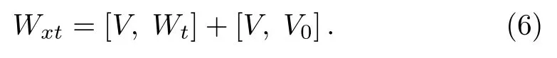
Equation(6)is referred to as matrix AKNS(?1)equation.By using Eq.(5),matrix AKNS(?1)equation(6)for the scalar functions u(x,t)and v(x,t)reads

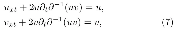
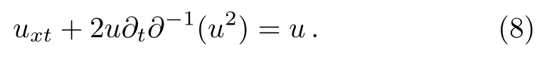
under the boundary conditions u→0,v→0 for|x|→∞.For u=v,Eq.(7)can be written as

And upon using u=ˉv in Eq.(7),one can obtain complex AKNS(?1)equation given by

It should be noted that in the case of the reductions u=v or u=ˉv,which are most important for applications(these reductions are considered in Sec.4,the system(2.6)reduces to well-studied equations.By use of the variable ω=(uv)introduced earlier,this system is written as

The elimination of ω brings to the system

For u=v,the further substitution ut=sinq brings to the sine-Gordon equation

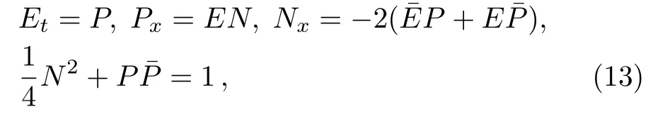
which coincide with the Maxwell-Bloch system,up to a scaling and interchange of x and t.

The solutions of the Lax pair(2)–(3)and Eq.(6)can be obtained by using DT.In the next section,we define DT by means of a Darrboux matrix on the solutions to the Lax pair and the solutions of the nonlinear evolution equation(6).

3 Darboux Transformation

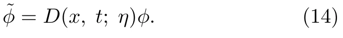
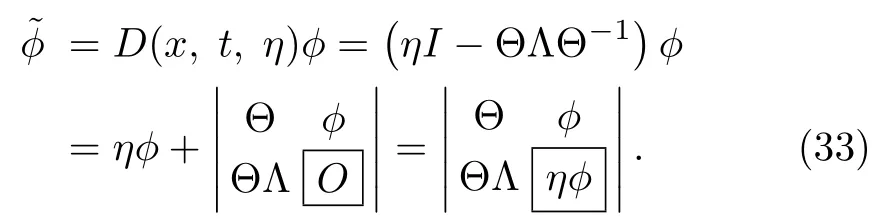
In what follows,we apply DT on the Lax pair(2)–(3)and the AKNS(?1)equation(6)to obtain soliton solutions.We define a DT on the solutions of the Lax pair equations(2)–(3)by means of a 2 × 2 Darboux matrix D(x,t;η).The Darboux matrix D(x,t;η)acts on the solution ? of the Lax pair(2)–(3)to give another solutioni.e.,

The covariance of the Lax pair(2)–(3)under the DT requires that the new solutionsatisfies the same Lax pair equations,but with the matricesi.e.,

with

where

To find a DT on the matrices,and.For this,we consider Darboux matrix to be

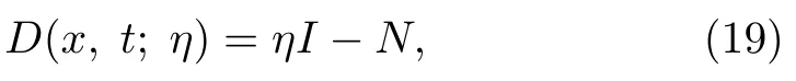
where I is the 2×2 identity matrix and N is the 2×2 auxiliary matrix,can be defined as

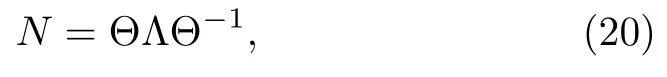
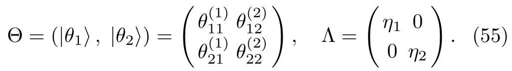
where Θ is the 2×2 particular matrix solution to the Lax pair(2)–(3),which is constructed by the eigen-matrix ? evaluated at different values of η,whereas the matrix Λ is a 2×2 diagonal matrix with eigenvalues η1, η2.Therefore,matrix Θ reads

In Eq.(21)|e1,|e2are the two constant column basis vectors,andin the matrix Θ is a column vector solution to the Lax pair(2)and(3).For η= ηi(i=1,2),we have

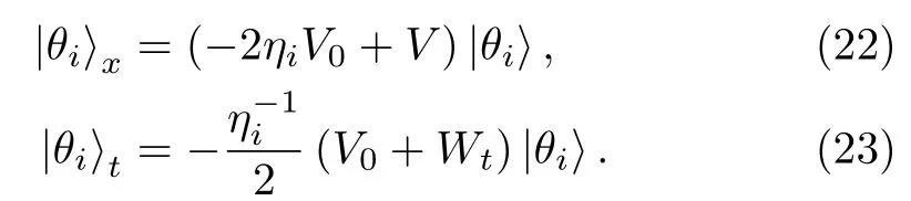
For Λ =diag(η1, η2),the Lax pair(22)–(23)can be written in matrix form as

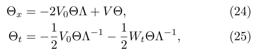
where Θ is a particular matrix solution to the Lax pair(2)–(3)at a particular eigen-value matrix Λ.

Based on the above findings,one can prove the following propositions.

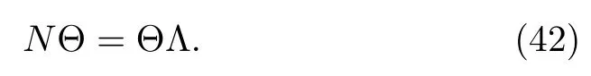
Proposition 1Under the DT(19),the new matrix solutionsandgiven in Eq.(18)have the same form as V in Eq.(5),provided the matrix N satisfies the following conditions

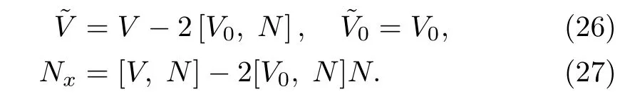
ProofThe relation betweenand V is established and given in Eq.(26).We now show that the choice of matrix N= ΘΛΘ?1satisfies the condition(27).For this,let us operate?xon the matrix N= ΘΛΘ?1and use Eq.(24),we have

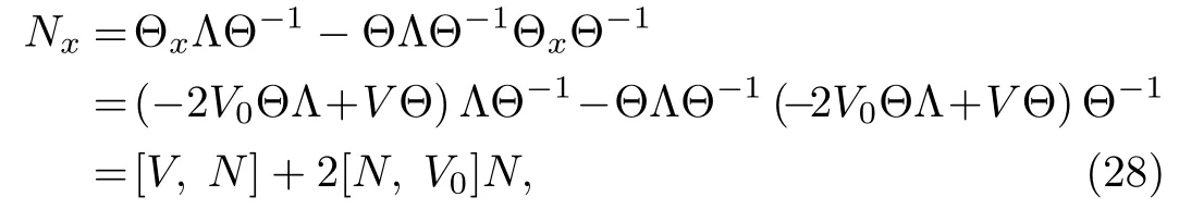
which is condition(27).Thus,the proof is complete.

Proposition 2The new solutionsandgiven by Eq.(18)have the same form as in Eq.(5),if the following conditions are ful filled

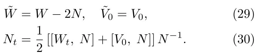
ProofTo proof the condition(30),let us operate?ton N= ΘΛΘ?1and use Eq.(25),we have

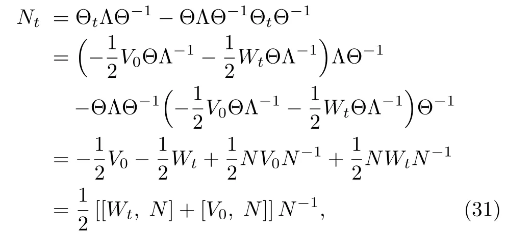
which is condition(30).This completes the proof.

Remark 1We remark here that Darboux transformation preserves the system i.e.,if ? and V,W,V0are respectively,the solutions of the Lax pair(2)–(3)and nonlinear evolution equation(6),then ?[K]and V[K],W[K],(that correspond to multi-soliton solutions)are also the solutions of the same equations.

In this paper,we will use quasideterminants that are expanded about q×q matrix.The quasideterminant expression of Q×Q expanded about q×q matrix is given as

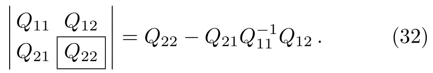
For details and properties see e.g.,Refs.[28]–[29].

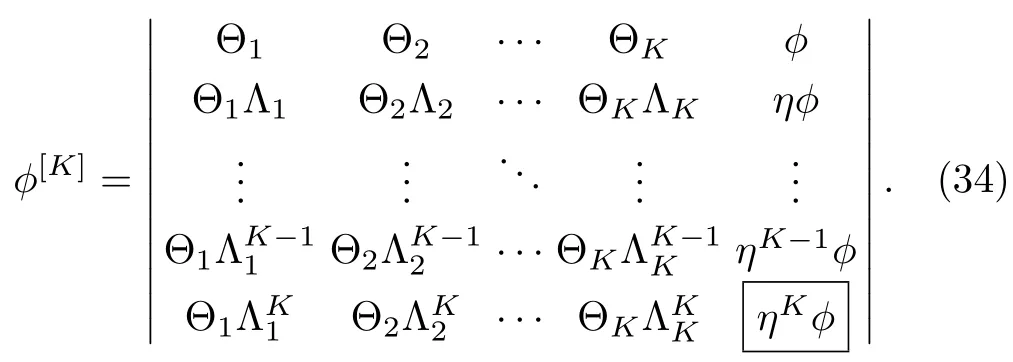
For N= ΘΛΘ?1,it seems appropriate here to express the solutions ?[K],V[K],,W[K]in terms of quasideterminants.The matrix solutionto the Lax pair(2)–(3)with the particular matrix solution Θ in terms of quasideterminant can be expressed as

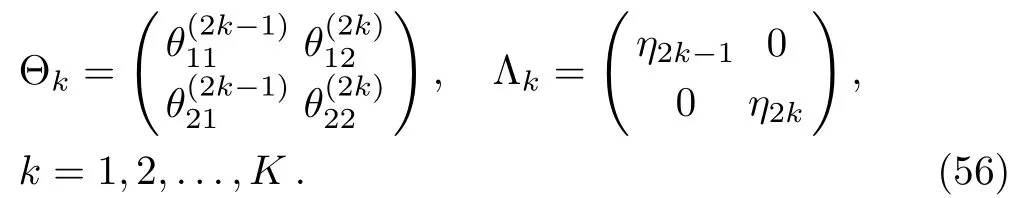
For the matrix solutions Θkat Λ = Λk(k=1,2,...,K)to the Lax pair(2)–(3),the K-times repeated DT ?[K]in terms of quasideterminant is written as(using the notation=?[1],Θ1=Θ,Λ1=Λ)

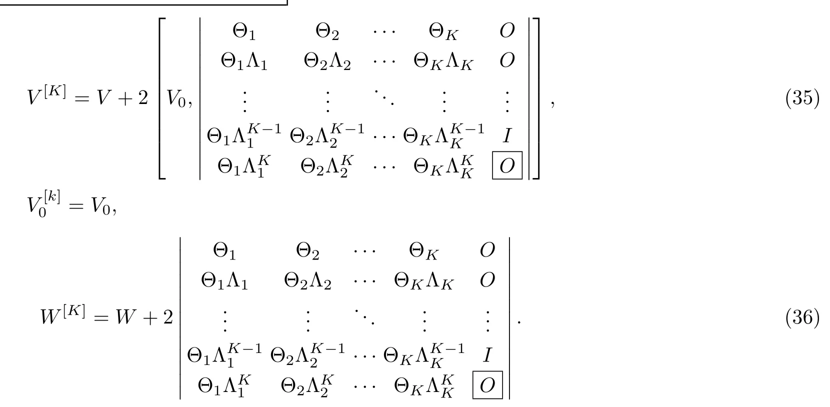
Similarly,the quasideterminant solutions V[K],,and W[K]can be expressed as

For an inductive proof of the obtained results similar to in Eqs.(34)–(36),reader is referred to see Ref.[18].The K-fold DT(34)can also be written in an appropriate form as

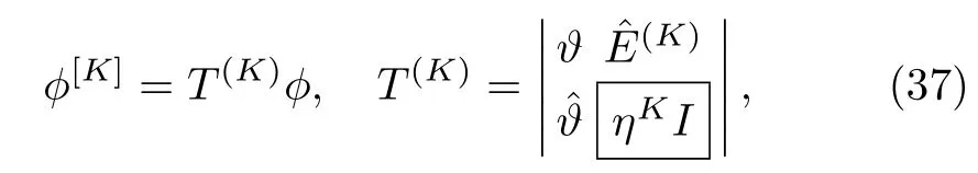
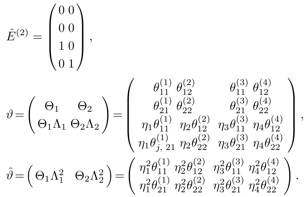
where T(K)is the 2×2 matrix,whereas,and ? are 2K×2,2×2K,and 2K×2K matrices respectively,given by

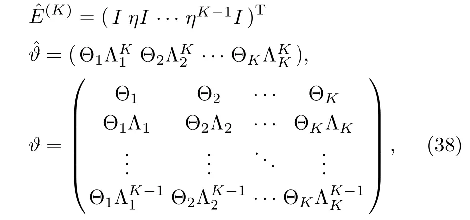
whereTrepresents usual transpose.Similarly,re-written the expression(36)as

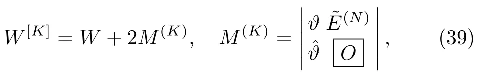
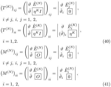
where M(K)is the 2×2 matrix andis the 2K×2 matrix.The components(or elements)of the matrices T(K)and M(K)can be decomposed as

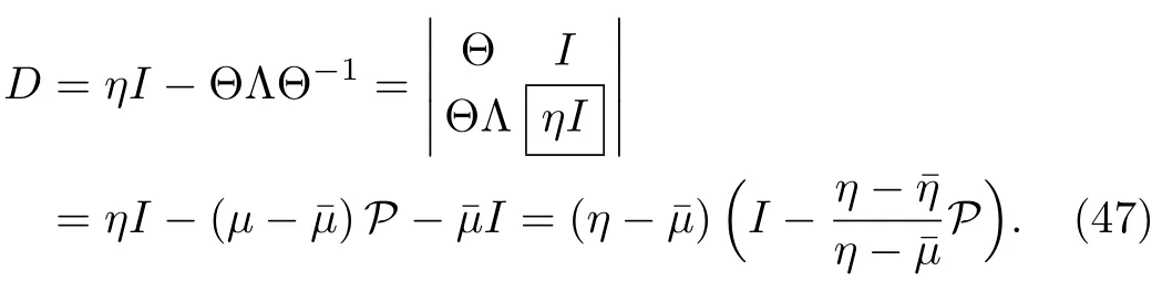
The quasideterminant solutions of the AKNS(?1)equation can also be related with the dressed solutions obtained by Darboux-dressing transformation.[30]In this method,matrix D referred to as dressing function(or Darboux-dressing matrix)is studied in the extended complex η-plane.The dressing function should be meromorphic in the complex plane i.e.it has some pole in the domain of η.It has a singular behavior at η= μ and can be expressed in terms of Hermitian projectors.To relate quasideterminant solutions with dressed solutions,we re-write the matrix N as

Let us define column solutions|θ1,|θ2of the Lax pair(2)–(3)at η = η1and η = η2(η1η2)respectively,then we have

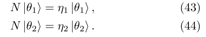
By taking η1=μ,η2=,we may write the matrix N in terms of superposition of Hermitian projectors i.e.,

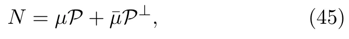
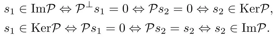
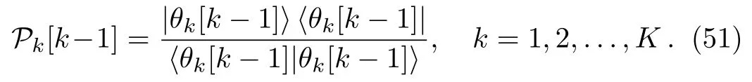
where P is a Hermitian projector that satisfy P2=P,P+P⊥=I.It should be noted that projector P can be completely described by the background of two subspaces S1=ImP spanned by the basis|eiand S2=KerP spanned by|ej(ij).This yields the following interpretation:

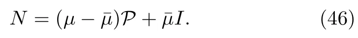
By using P⊥=I?P in Eq.(45),we have

Now Darboux matrix D in terms of Hermitian projector can be written as

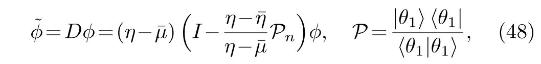
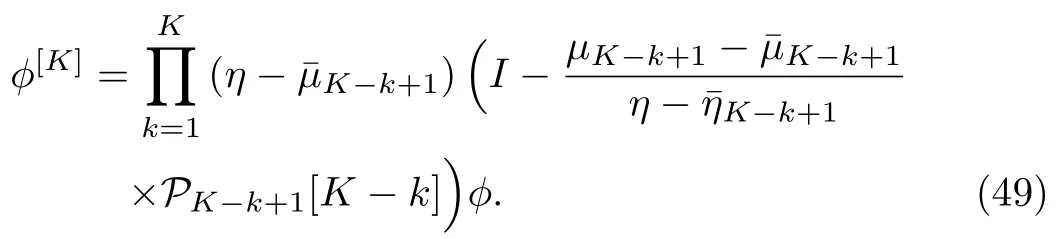
where|θ1is the column vector solution to the Lax pair(2)–(3).The K-times repeated DT on the matrix ?[K]in terms of Hermitian projector can be written as

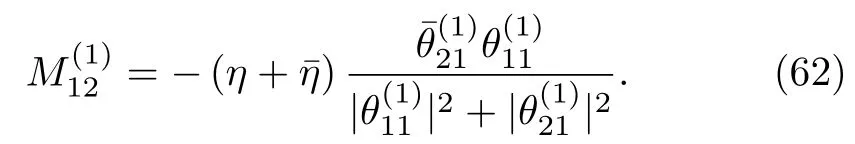
Similarly,the expression for W[K]in terms of Hermitian projector is

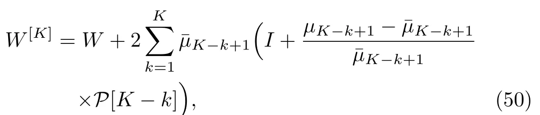
where

In the same way,one can also write expression for V[K],in terms of P.

4 Soliton Solutions

In this section,we shall discuss two cases i.e.,(u=reduction)that correspond to complex AKNS(?1)equation(9)and(u=v reduction)that correspond to Eq.(8)and compute explicitly one-,two-,and three-soliton solutions for both of the equations.In order to obtain soliton solution,let us take u=v=0 as a trivial solution,so that the Lax pair(2)–(3)with this seed(or trivial solution)are written as

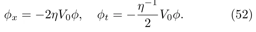
Equation(52)is satisfied if

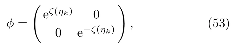
where ζ(ηk)= ηkx+(1/4ηk)t+ ηk0,k=1,...,K.

4.1 u= Reduction

In what follows,by expanding quasideterminant Darboux matrix,we express DTs on the solutions to the complex AKNS(?1)equation as a ratio of determinants.

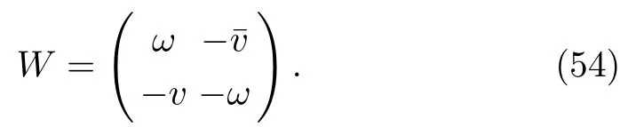
For a complex AKNS(?1)equation(9),matrix W in Eq.(5)takes the form

The particular matrix solution Θ to the Lax pair of the complex AKNS(?1)equation can be written as

By iterating particular matrix Θ to K-times,one can obtain the multi solutions to the Lax pair of the complex AKNS(?1)equation.For k=1,2,...,K,Eq.(55)reads

From Eqs.(39)and(54),we obtain the K-fold DTs to the solutions of the complex AKNS(?1)equation given by

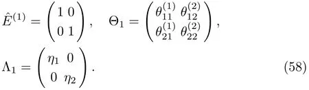
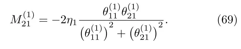
It may be noted that,from Eq.(35)one can find the same results for the DT on the solutions of the complex AKNS(?1)equation as in Eq.(57).To get one-soliton solution let us take K=1,so that the matrices(1),Θ1,Λ1are written as

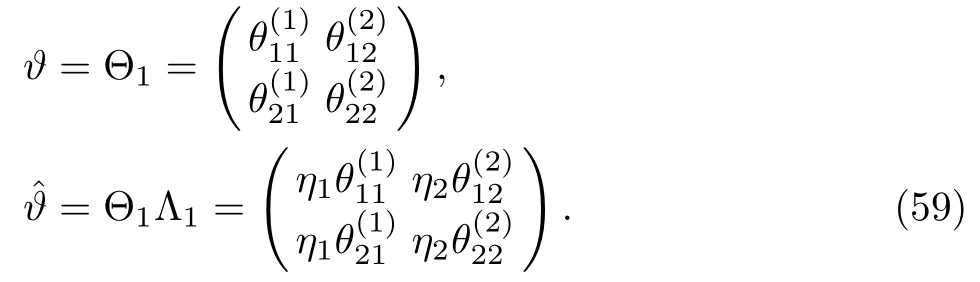
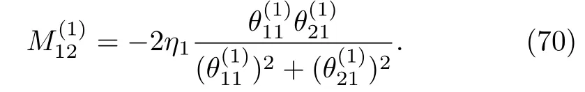
Therefore the matrix elementin the matrix M(1)can be computed as

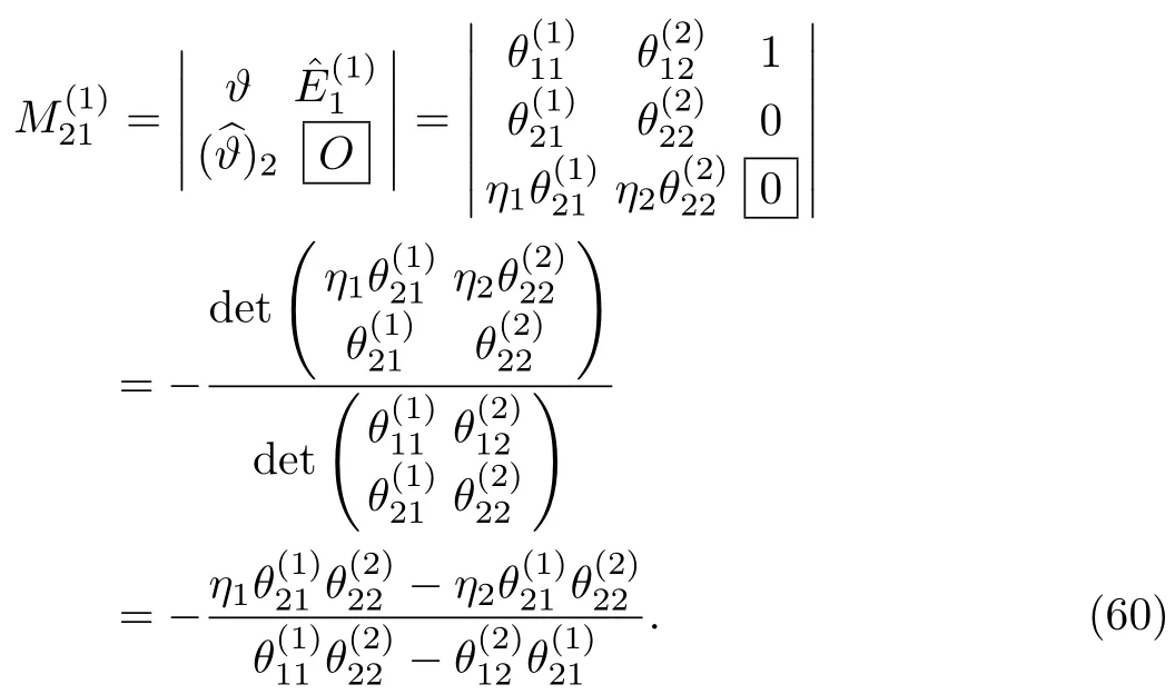
Similarly,

From Eqs.(61)and(62),it can be verified that=.Using Eq.(53),particular matrix solution to the Lax pair of the complex AKNS(?1)equation is given by

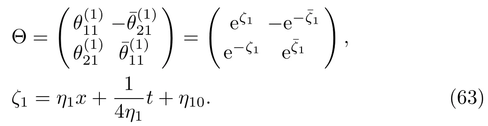
By using Eqs.(61)and(63)in Eq.(57),we obtain

The solution(64)is plotted in Fig.1.For two-soliton K=2,the matrices(2),?,being 4×2,4×4,2×4 respectively,to be taken as follow

The two-fold DT on the solution to the complex AKNS(?1)equation is

Similarly,one can also expressas a ratio of two determinants.By substitutingin Eqs.(65)with(66),we obtain two-soliton solution to the complex AKNS(?1)equation(9).The two-soliton solutions are depicted in Figs.2 and 3.

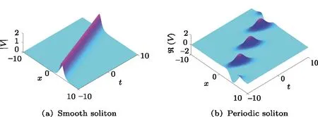
Fig.1 (Color online)One-soliton solution to the complex AKNS(?1)equation(9)with the choice of parameters:η1=0.5 ?0.5i,η10=0.

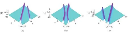
Fig.2 (Color online)Two-soliton solution to the complex AKNS(?1)equation for the choice of parameters: η1=?0.4?0.4i,η2=0.3+0.3i.

In Fig.2(a)for η10=0, η20= ?5,it can be seen that two solitons traveling parallel and are far from each other with their respective shapes and motions.However,when η10=0, η20=0(Fig.2(b)),soliton with the shorter amplitude interact elastically with other soliton having taller amplitude and both of them are trying to exchange their energies,while in Fig.2(c)for η10=0, η20=5,two solitons recover their respective original profiles and move parallel far from to each other as the beginning.Similar phenomena is observed for periodic solitons Figs.3(a)–(3c).

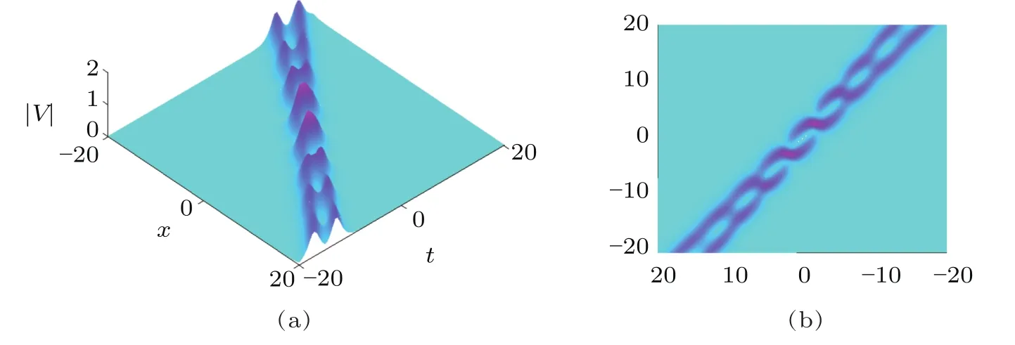
Fig.4 (Color online)Scattering of two solitons with the velocities nearby close to each other.

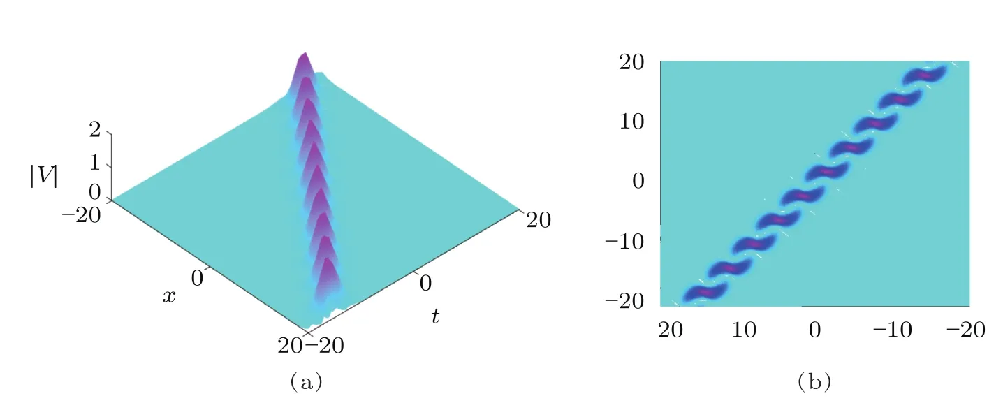
Fig.5 (Color online)Scattering of two solitons with the same velocities.

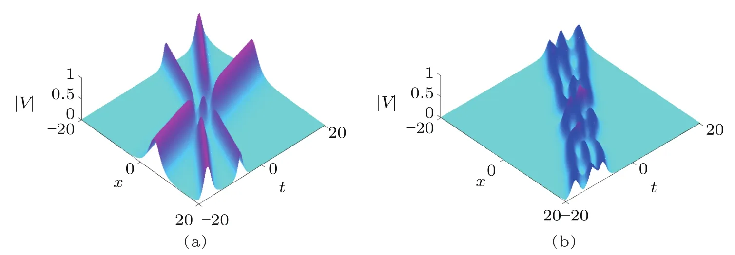
Fig.6 (Color online)(a)shows scattering of three solitons with their relative velocities,while(b)shows scattering of three solitons with the velocities are close to each other for Eq.(9).

We now consider another configuration of two soliton solution that has been shown in Figs.4 and 5.In Figs.4 and 5,we observe different effects of two-soliton solution to the complex AKNS(?1)equation with respect to particular values of their spectral parameters.Figure 4 shows the interaction between two solitons propagating with the velocities nearby close to each other.Figure 5 depicts the interaction of two solitons with their bound states having the same velocities(i.e.,?z=z1?z2=0,where z represents the velocity of each soliton).The bright area means the amplitude is largest,while the area with the cyanic background shows the amplitude is nearly to zero.Three-soliton solution numerically is shown in Fig.6.

4.2 u=v Reduction

For u=v,matrix W in Eq.(5)takes the form

The K-fold DT to the solution of the AKNS(?1)equation(8)yields

Similarly

Equations(69)and(70)imply that.By using Eq.(69)in Eq.(68),one-soliton(K=1)solution to the AKNS(?1)equation(8)given by

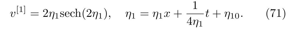
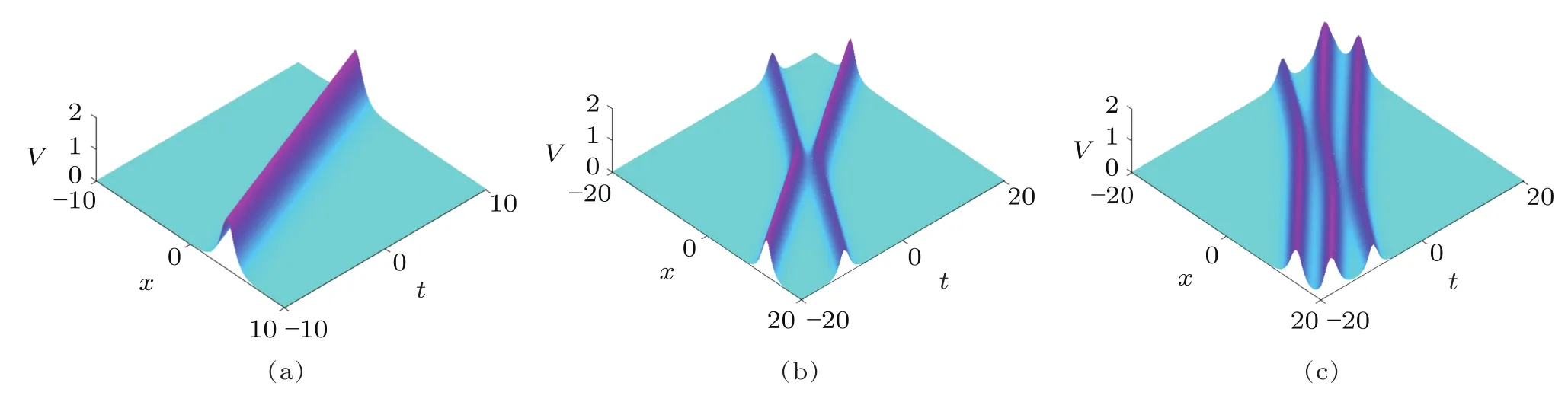
Fig.7 (Color online)One-,two-,and three-soliton solutions to the AKNS(?1)equation(8).

The asymptotic limit i.e.,when t→ ∞,we have ζ→∞,Eq.(71)becomes

So we get the much simpler expression of the onesoliton solution in the asymptotic limit.Similarly,K-soliton solution in the asymptotic limit reads

5 Concluding Remarks

In this paper,we have discussed Darboux transformation for a negative order AKNS equation.Using quasideterminant Darboux matrix,we have computed multisoliton solutions of the AKNS(?1)equation.The K-soliton solutions have been expressed in simple quasideterminant form through iteration process and shown to be related with the dressed solutions as obtained by dressing method.As an example,we have presented one-,two-,and threesoliton solutions of the AKNS(?1)equation.It has also been shown that,each envelope soliton able to resume its original shape after collision,which shows that collision between envelope solitons is elastic collision.It would be interesting to study the discrete,semi-discrete and supersymmetric generalization of the model via Darboux transformation.