High-Order Lump-Type Solutions and Their Interaction Solutions to a(3+1)-Dimensional Nonlinear Evolution Equation?

Tao Fang(方濤),Hui Wang(王惠),,2,? Yun-Hu Wang(王云虎),,3and Wen-Xiu Ma(馬文秀)

1College of Art and Sciences,Shanghai Maritime University,Shanghai 201306,China

2Department of Mathematics and Statistics,University of South Florida,Tampa,FL 33620,USA

3Department of Mathematics and Information Technology,The Education University of Hong Kong,Hong Kong,China

4Department of Mathematics,King Abdulaziz University,Jeddah,Saudi Arabia

5College of Mathematics and System Science,Shandong University of Science and Technology,Qingdao 266590,China

6Department of Mathematical Sciences,North-West University,Ma fi keng Campus,Mmabatho 2735,South Africa

AbstractBy means of the Hirota bilinear method and symbolic computation,high-order lump-type solutions and a kind of interaction solutions are presented for a(3+1)-dimensional nonlinear evolution equation.The high-order lumptype solutions of the associated Hirota bilinear equation are presented,which is a kind of positive quartic-quadraticfunction solution.At the same time,the interaction solutions can also be obtained,which are linear combination solutions of quartic-quadratic-functions and hyperbolic cosine functions.Physical properties and dynamical structures of two classes of the presented solutions are demonstrated in detail by their graphs.

Key words:high-order lump-type solutions,interaction solutions,Hirota bilinear method

1 Introduction

The investigation of rational solutions on nonlinear evolution equations(NLEEs)has attracted much attention from mathematicians,physicists,and many scientists in other fields.Among these rational solutions,[1]lump solutions and rogue wave solutions have been found in many integrable systems.[2?7]Recently,the study of lump solutions,which rationally localized in all directions in the space,becomes a hot topic in soliton theory.[8?22]Over the past decades,many powerful methods have been developed to find the lump solutions of NLEEs,such as the Hirota bilinear method,[23]the long wave limit approach,[3]and the nonlinear superposition formulae.[24]Among these methods,the Hirota bilinear method is a direct method,which can be used to obtain the exact solutions for NLEEs once its corresponding bilinear form is given.By taking the function f in the bilinear equation as a positive quadratic function,Ref.[8]obtained the lump solutions of the KPI equation,which can be reduced to the ones in Refs.[3,25].Then,this method is widely used to find lump solutions or lump-type solutions for generalized fifth-order KdV equation,Boussinesq equation,(4+1)-dimensional Fokas equation and so on.[11?21]References[26?44]further extended this method to find interaction solutions for integrable and non-integrable system.

In this paper,we focus on the following(3+1)-dimensional NLEE

Through the dependent variable transformation

Eq.(1)is transformed into the Hirota bilinear form

where the derivatives Dy,DxDz,and DyDtare the bilinear operators defined by[23]

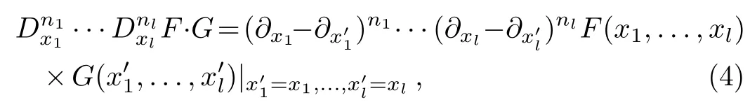
and the corresponding bilinear form of Eq.(3)equals to

The structure of this paper is as follows.In Sec.2,high-order lump-type solutions are constructed by using the Hirota bilinear method,which are obtained by taking function f in Eq.(3)as a kind of positive quarticquadratic-functions.In Sec.3,a kind of interaction solutions are derived by assuming function f in Eq.(3)as a combination of positive quartic-quadratic-functions and hyperbolic cosine functions.Finally,some conclusions will be given in Sec.4.

2 High-Order Lump-Type Solutions for Eq.(1)

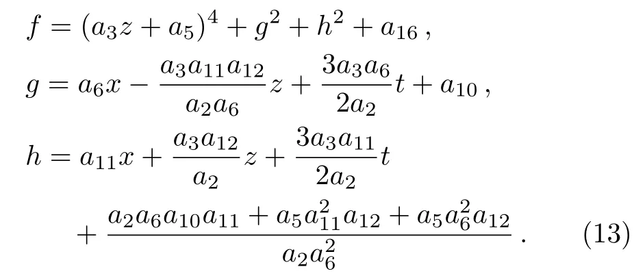
In this section,we will construct high-order lump-type solutions of Eq.(1)by taking f in Eq.(3)as a combination of positive quartic-quadratic-functions

with

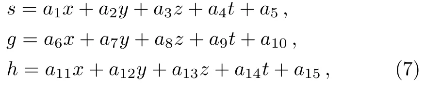
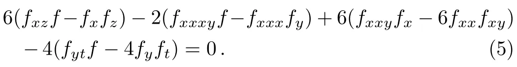
where the real parameters ai(1≤i≤16)will be determined later.Substituting ansatz(6)with(7)into Eq.(3)with a direct symbolic computation,it generates the following results

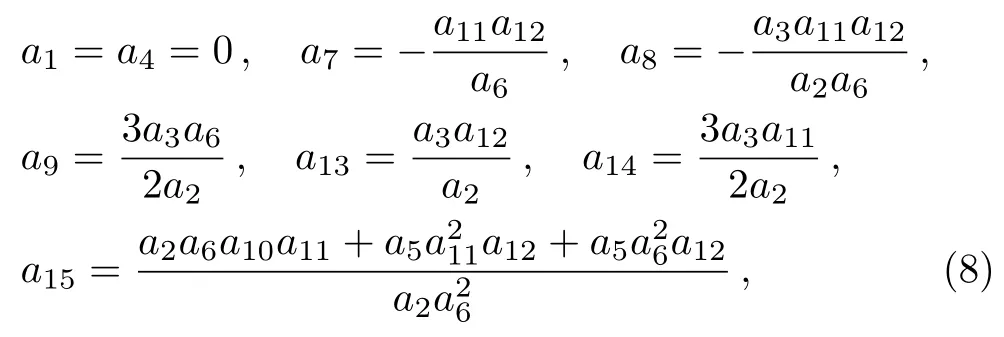
which need to satisfy constraint conditions as follows

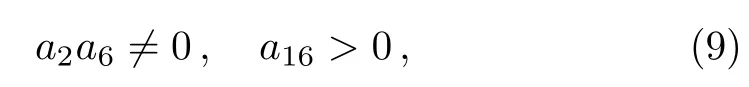
to ensure the corresponding solution f is well defined.With the constraint conditions(9)and transformation(2),the solution(6)can be obtained as follows

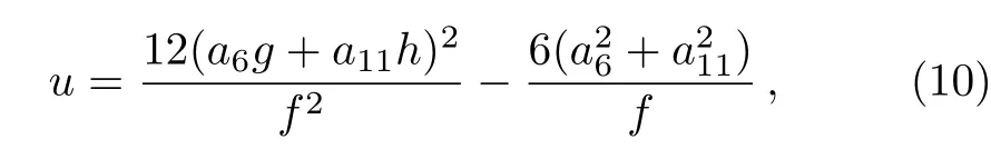
where

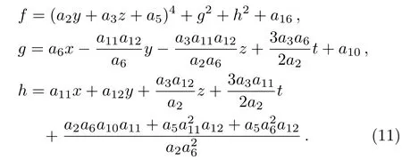
Case 1By taking y=0,the solution(10)can be reduced to the following form

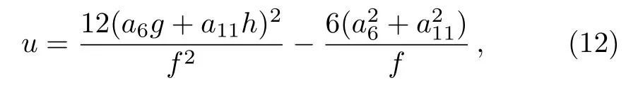
with

It is easy to calculate that there are three critical points to solution(12),which reads

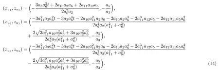
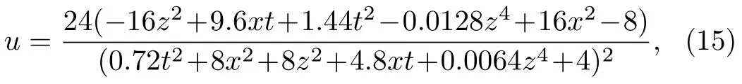
In order to show the physical properties and structures of solutions(12)more clearly,we select the parameters as a2=1,a3=0.2,a5=0,a6=1,a10=1,a11=1,a12=5,a16=1,which yields

and the corresponding three critical points can be further calculated as follows

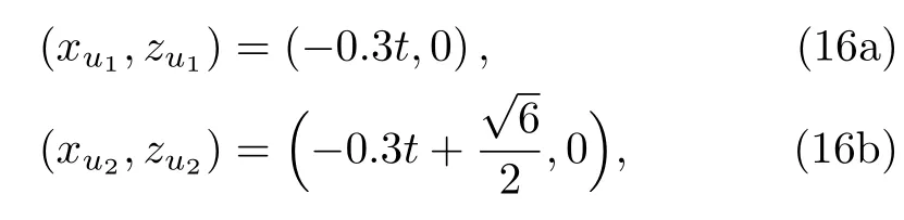
It is easy to found that solution(15)has a local minimum value umin= ?12 at(?0.3t,0)and a local maximum valueand,which can be clearly observed from Fig.1.Figure 2 is the corresponding density-plots in the(x,z)-plane when t=?10,0,10,respectively.

Case 2By taking z=0,the solution(10)can be reduced to the following form

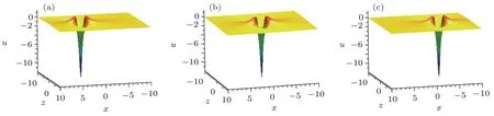
Fig.1 (Color online)Evolution plots of the solution(15).(a)t=?10,(b)t=0,(c)t=10.

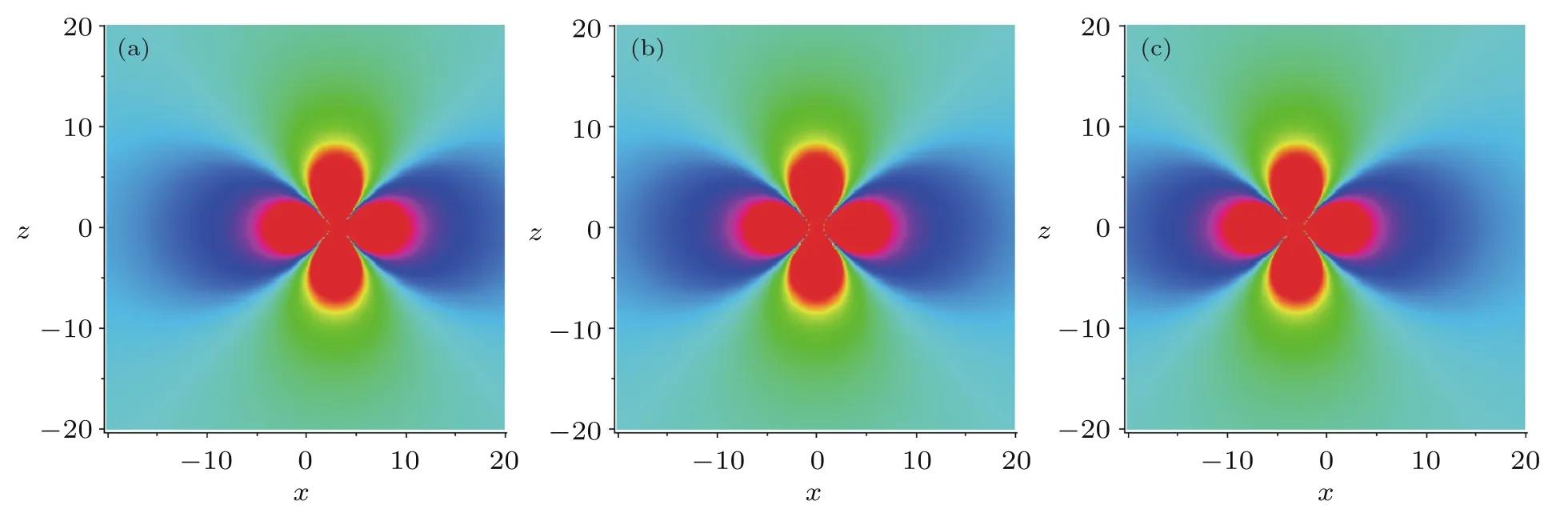
Fig.2 (Color online)Corresponding density plots for Fig.1.(a)t=?10,(b)t=0,(c)t=10.

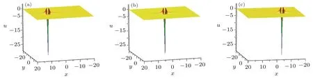
Fig.3 (Color online)Evolution plots of the solution(20).(a)t=?10,(b)t=0,(c)t=10.

where

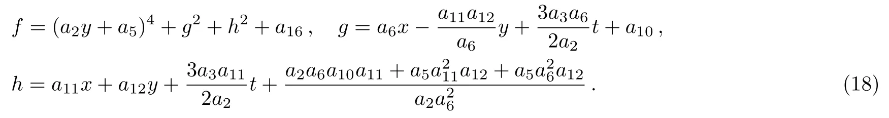
It is easy to find that solution(17)also has three critical points

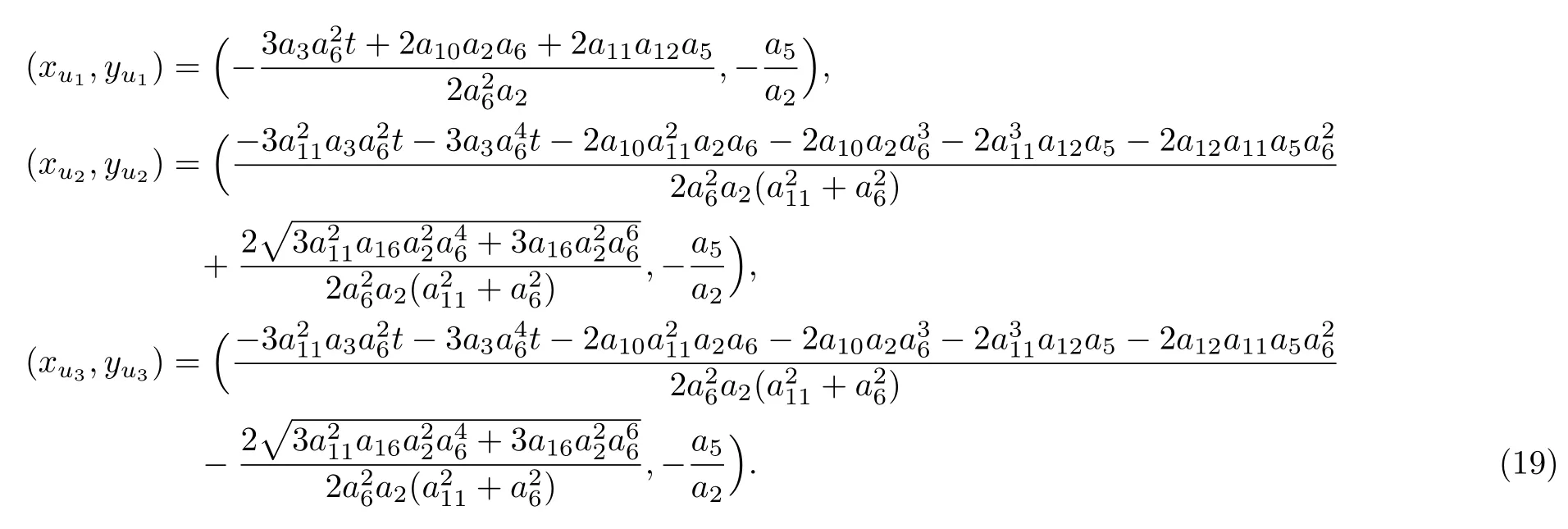
By taking the corresponding parameters as a2=1,a3=0.2,a5=0,a6=1,a10=1,a11=1,a12=5,a16=1,solution(17)with(18)can be reduced to the following form

and the corresponding three critical points reads

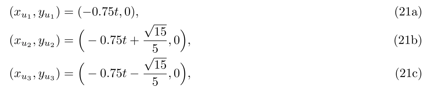
which point(?0.75t,0)corresponds to a local minimum value umin= ?30,and points(?0.75t±(/5),0)correspond to a local maximum value umax=3.75.For the corresponding 3D-plots and density-plots,see Figs.3 and 4.

Case 3When x=0 and a5=0,one can see that g and h in Eq.(11)satisfy g=?(a11/a6)h,which means expression(6)can be rewritten as f=s4+(1+α2)h2+a16.Unfortunately,f=s4+(1+α2)h2+a16will lead to solution u is not localized in all directions in space.[13,41]

By choosing appropriate parameters with a2=2,a3=1,a5=0,a6=2,a10=0,a11=1,a12=1,a16=1,x=0,one can simplify solution(10)to the following form

which corresponding 3D-plots and density-plots can be seen in Figs.5 and 6.

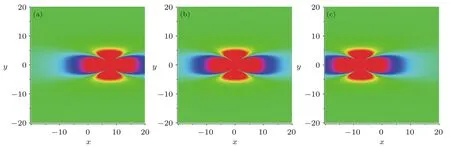
Fig.4 (Color online)Corresponding density plots for Fig.3.(a)t=?10,(b)t=0,(c)t=10.

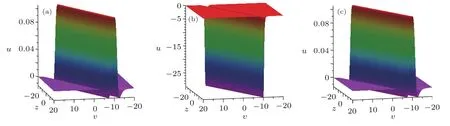
Fig.5 (Color online)Evolution plots of the solution(22).(a)t=?10,(b)t=0,(c)t=10.

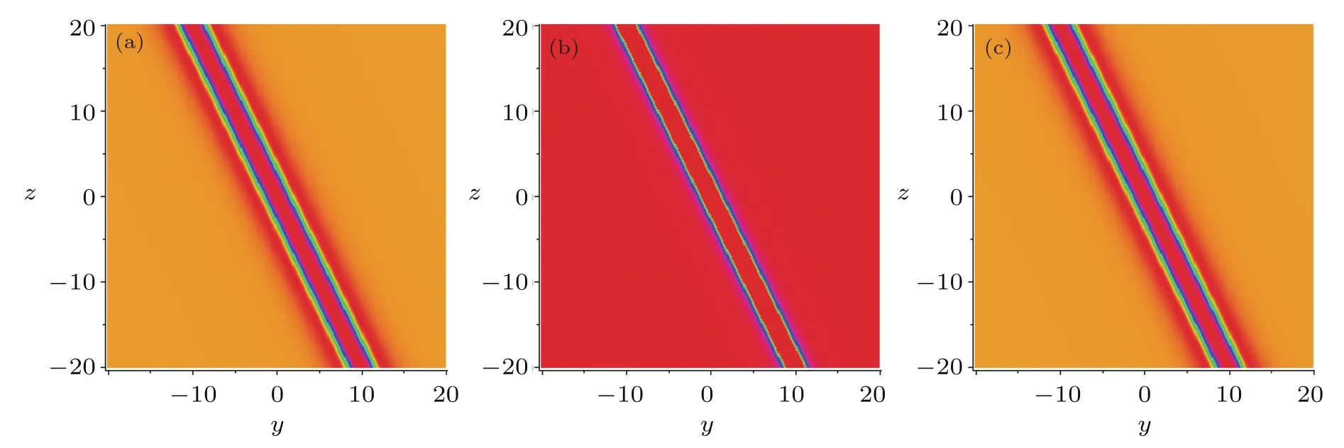
Fig.6 (Color online)Corresponding density plots for Fig.5.(a)t=?10,(b)t=0,(c)t=10.

3 A Kind of Interaction Solutions for Eq.(1)

In order to find the interaction solutions to Eq.(1),the function f in Eq.(3)may be taken as the following form

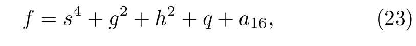
with

where the real parameters ai(1≤i≤16)and k,kj(1≤j≤4)are all to be determined later.Substituting ansatz(23)with(24)into Eq.(3),we obtain

which need to satisfy the following constraint conditions

to ensure the corresponding solution u is positive,analytical and localized in all directions in the(x,y,z)-plane.With the conditions(25)and(26),the solution of Eq.(1)can be obtained as follows

with

Case 1Taking a2=0.5,a3=2,a8=1,a10=0,a13=1,a15=0,a16=2,k=5,k1=2,y=0,solution(27)can be reduced to the following form

which corresponding 3D-plots and density-plots can be seen in Figs.7 and 8.

Case 2By selecting the parameters as a2=1,a3=2,a8=4,a10=0,a13=2,a15=0,a16=1,k=4,k1=2,z=0,solution(27)can be rewritten as

which corresponding 3D-plots and density-plots can be seen in Figs.9 and 10.From Figs.7,8,9,and 10,it can be clearly seen that the above two types of solutions(29)and(30)can be regarded as“soliton” solutions.

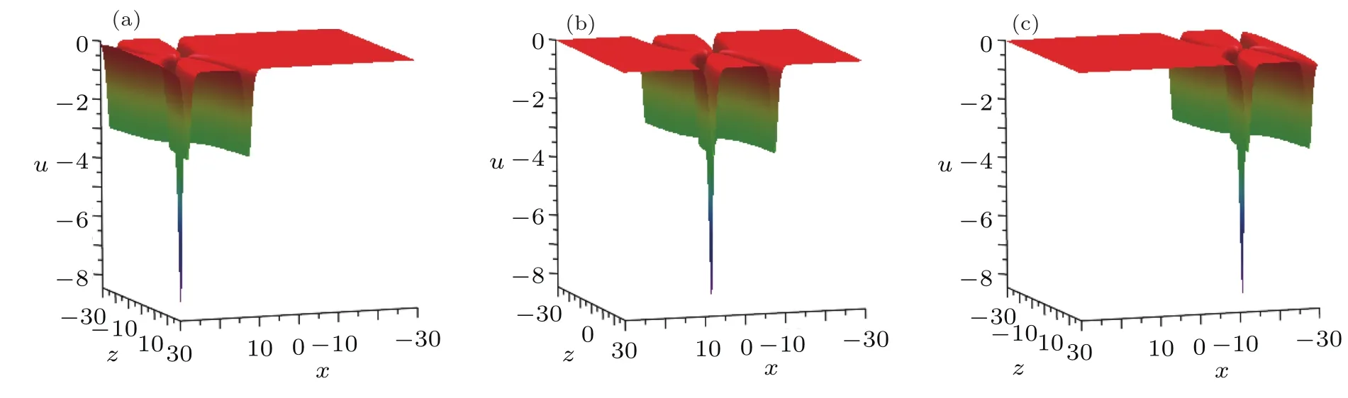
Fig.7 (Color online)Evolution plots of the solution(27).(a)t=?5,(b)t=0,(c)t=5.

Fig.8 (Color online)Corresponding density plot for Fig.7.(a)t=?5,(b)t=0,(c)t=5.

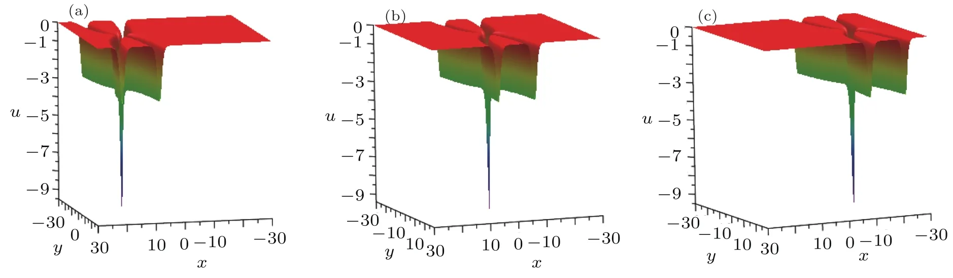
Fig.9 (Color online)Evolution plots of the solution(30).(a)t=?15,(b)t=0,(c)t=15.

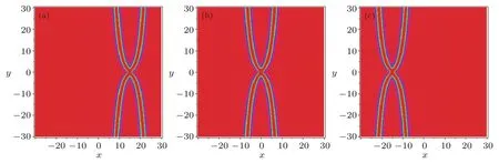
Fig.10 (Color online)Corresponding density plot for Fig.9.(a)t=?15,(b)t=0,(c)t=15.

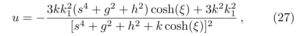
Case 3By choosing appropriate parameters with a2=0.5,a3=1,a8=2,a10=0,a13=2,a15=0,a16=2,k=5,k1=2,x=0,solution(27)reads

Figures 11 and 12 show the interaction phenomenon,which is induced by the twin-strip solitons for solution(31).Figures 11(a)and 12(a)show there are two stripe solitions at the time t=?3,and when t=0,the two stripes solitons disappear and one stripe soliton appears which has much more energy and higher peak that one can see in Figs.11(b)and 12(b),as time goes by,the twin-strip solitons start appearing which can be seen in Figs.11(c)and 12(c).In fact,in expression(28),h= βg when a13= βa8,a15= βa10,which means the function f in Eq.(23)could be rewritten as f=s4+(1+ β2)g2+cosh(γt)under x=0.From Sec.2,the function f=s4+(1+β2)g2yields lump-type solution along the direction of x=0.It is obvious that when t=0 there is no cosh(γt)but only lump-type soliton,and when t=0,there are twin-stripe solitons.

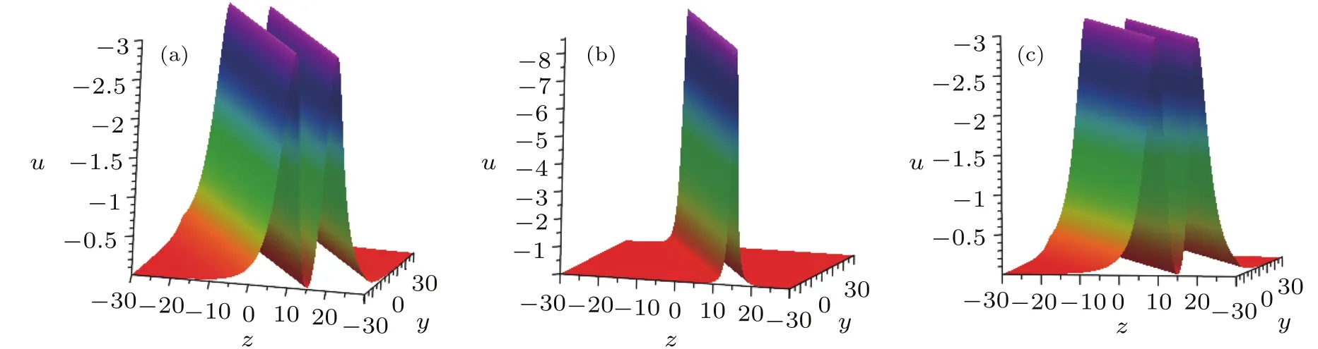
Fig.11 (Color online)Evolution plots of the solution(31).(a)t=?3,(b)t=0,(c)t=3.

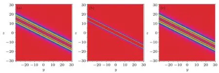
Fig.12 (Color online)Corresponding density plot for Fig.11.(a)t=?3,(b)t=0,(c)t=3.

4 Conclusions

In summary,by using the means of the Hirota direct method and symbolic computation,the high-order lump-type solutions(10)and their interaction solutions(27)to the(3+1)-dimensional nonlinear evolution equation(1)are studied.By taking the function f in Hirota bilinear equation(3)as a kind of positive quartic-quadratic-functions,the high-order lump-type solutions(10)are constructed which the dynamic mechanism can be seen in Figs.1–6.Furthermore,when we take the f as a combination of positive quartic-quadratic-functions and hyperbolic cosine functions,the interaction solutions(27)are presented,and their corresponding dynamic physical properties are vividly showed in Figs.7–12.

Conflict of Interest

The authors declare that they have no con fl ict of interest.