SANG Xiaoyan(桑小艷),JIANG Guo(姜國) WU Jieheng(吳介恒),LU Yiyang(盧逸揚(yáng))

(1.School of Mathematics and Statistics,Hubei Normal University,Huangshi 435002,China;2.Department of Mathematics,Vanderbilt University,Nashville,Tennessee 37253,USA)

Abstract: This article introduces an efficient numerical method on the base of block pulse functions to solve nonlinear stochastic It?-Volterra integral equations.Integral operator matrix of block pulse functions is used to transform the nonlinear stochastic integral equations into a set of algebraic equations.Moreover,we give error analysis and prove that the rate of convergence of this method is fast.Lastly,some numerical examples are given to support the method.

Key words: Block pulse function;Integration operational matrix;Stochastic It?-Volterra integral equation

1.Introduction

Volterra integral equations which rise from physical and chemistry have been studied widely.Nowadays,stochastic Volterra integral equations have also been applied in many fields such as mechanics,medicine,biology,finance,social science and so on.These systems often rely on Gaussian white noise.As we all know,stochastic Volterra integral equations usually cannot be solved explicitly.So,it is important to provide the numerical solutions of these equations.There has been a growing interest in numerical solutions to different Volterra integral equations for a long time.Different orthogonal basis functions,polynomials or wavelets,such as block pulse functions,Fourier series,Walsh functions,Legendre polynomials,Chebyshev polynomials,Haar wavelet,etc.,are used to estimate the solutions of different Volterra integral equations.Here we only mention [1,4,5,8-12,14,16-17],the details can refer to other relevant literatures.

In specially,Maleknejad et al.[10]and Fakhrodin[12]studied the following linear stochastic Volterra integral equation:

whereu(t),f(t),(s,t)and(s,t)are the stochastic processes defined on the probability space(?,F,P)fors,t∈[0,T),andu(t)is unknown stochastic function.B(t)is a Brownian motion and the second integral term is It? integral.The authors transform stochastic Volterra integral equation to algebra equation by block pulse function and Haar wavelet respectively and give the numerical solutions to the equations.Similarly,Maleknejad et al.[6]obtained a numerical method for stochastic Volterra integral equation driven bymdifferent Brownian motions.Moreover,on the base of modified block pulse functions,Maleknejad et al.[7]presented a new technique for solving the above integral equation.The rate of convergence of the method is faster than the one based on block pulse functions.Ezzati et al.[15]proposed an efficient numerical method to linear stochastic Volterra integral equation driven by fractional Brownian motion andnindependent one-dimensional standard Brownian motions based on block pulse functions.

For nonlinear stochastic integral equation,Asgari et al.[11]presented a practical and computational numerical method by means of Bernstein polynomials.By the generalized hat functions,Heydari et al.[13]provided the numerical solution to the following nonlinear equation

whereu(t),f(t),andare the stochastic processes defined on the probability space(?,F,P) fors,t∈[0,T),andu(t) is an unknown stochastic function.The second integral term is It? integral.σandgare analytic functions.The authors reveal the accuracy and efficiency of the method by some examples,but,the rate of convergence to the numerical solution cannot be given.Moreover,in line with the same hat functions,Hashemi et al.[2]also presented the numerical method of the above nonlinear stochastic integral equation driven by fractional Brownian motion.In a general way,ZHANG[18?19]studied the existence and uniqueness solution to stochastic Volterra integral equations with singular kernels and construct a Euler type approximate solution.

However,as far as we know,there are still few papers about the numerical solutions to the following nonlinear stochastic It?-Volterra integral equation

whereu0(t)is known determinate function,andare determinate kernel functions defined on 0

In Section 2,we recall the definition and properties of block pulse functions.In Section 3 and 4,we show the integral and stochastic integral operator matrices about block pulse functions respectively.In Section 5,the error and the rate of convergence of this method are given.In Section 6,an efficient numerical method to nonlinear integral equation (1.3) is obtained.In Section 7,some numerical examples illustrate the validity of the method.

2.Block Pulse Functions and Function approximation

Block pulse functions (BPFs) have been widely learned by lots of scholars and applied to solve different problems.For example,[10]gives a detailed description.This section first recalls the notation and definition of BPFs.BPFs are defined as

wheret∈[0,1),i=1,2,···,mandh=

There are some basic properties of BPFs as follows

(i) Disjointness:

wheret∈[0,1),i,j=1,2,···,mandδijis Kronecker delta;

(ii) Orthogonality:

(iii) Completeness:for everyf∈L2[0,1),Parseval’s identity holds:

where

The set of BPFs can be written as a vector of dimensionm:

From the above description and properties,it follows that:

whereFm=(f1,f2,···,fm)T,

It is also easy to show that

whereGis am×mmatrix andis a vector with elements equal to the diagonal entries ofG.

Any functionu(t)∈L2([0,1)) can be expanded as

whereum(t) is the approximation of BPFs ofu(t),m=2αfor a positive integerα.Cmis the block pulse coefficient vector as

Letk(s,t)∈L2([0,1)×[0,1)).It can be expanded as following

whereΘm1(s) andΛm2(t) are respectivelym1andm2dimensional block pulse coefficient vectors,K=(kij),i=1,2,···,m1,j=1,2,···,m2,which is them1× m2block pulse coefficient matrix,and

h1=h2=For the sake of convenience,we setm1=m2=m.

3.Integration Operational Matrix

This section recall some integration operational matrices(for the details,see [10])

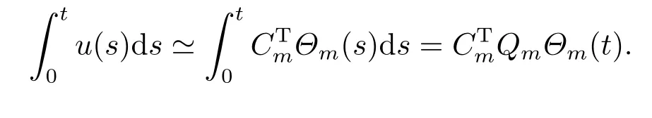
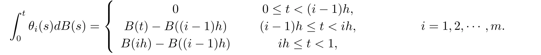
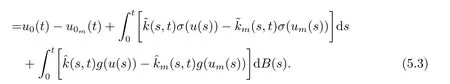
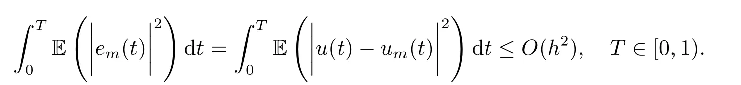
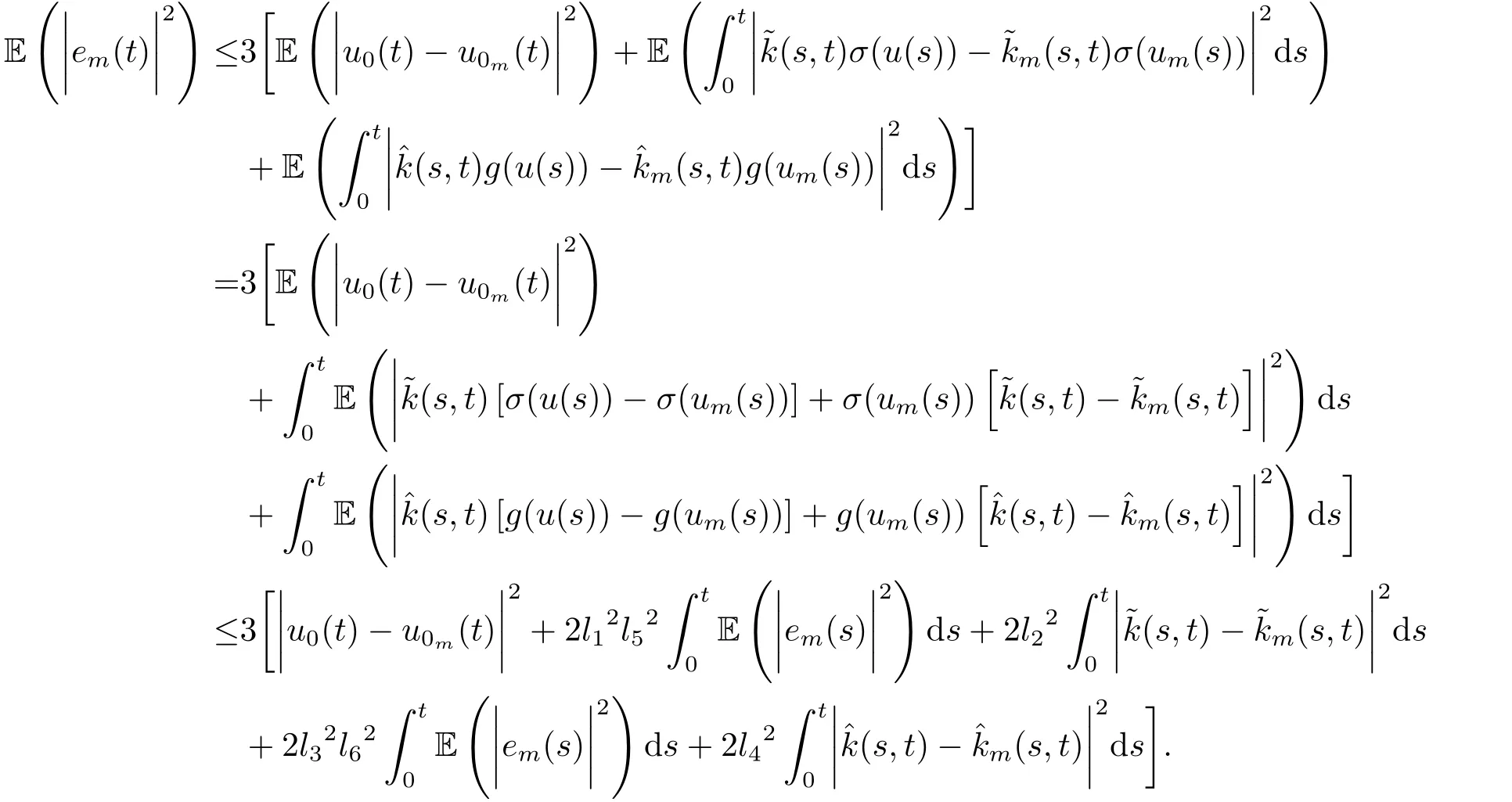
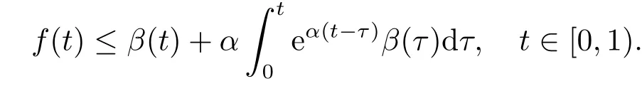
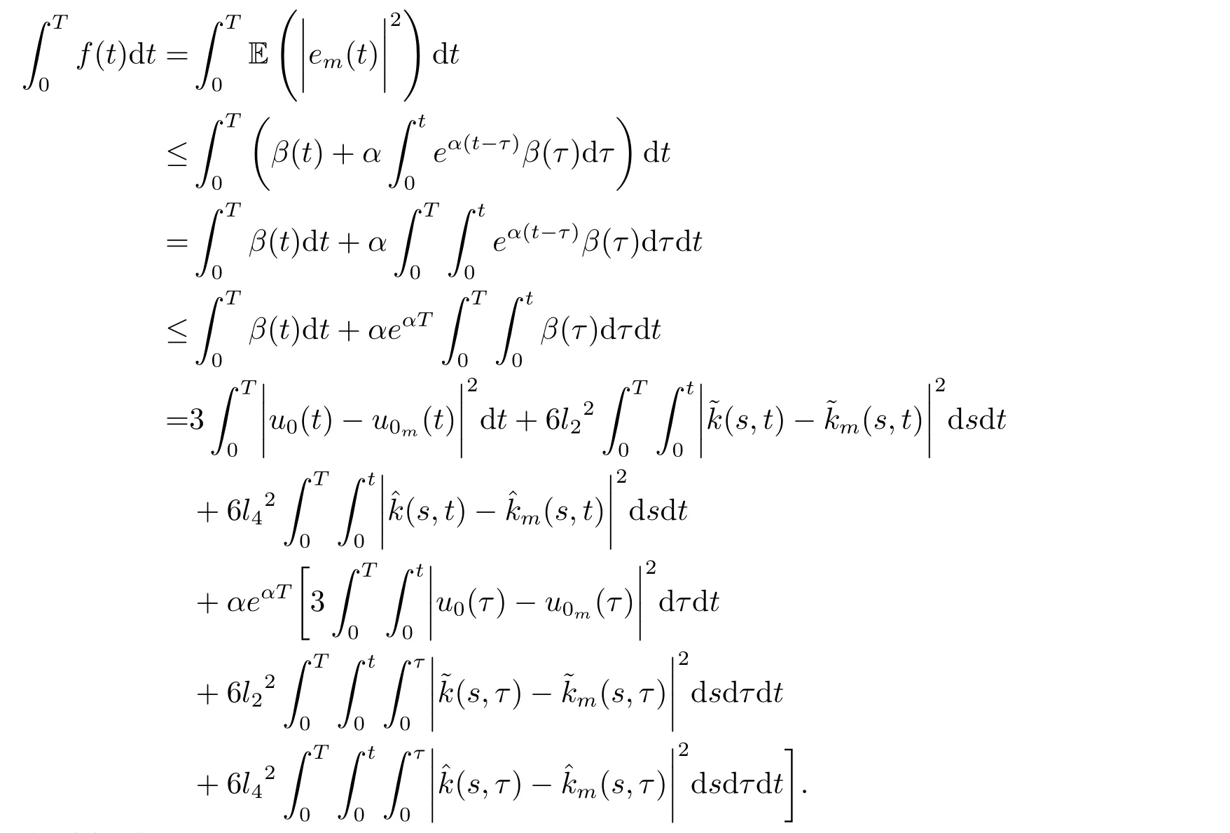
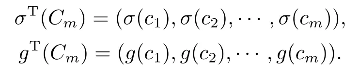
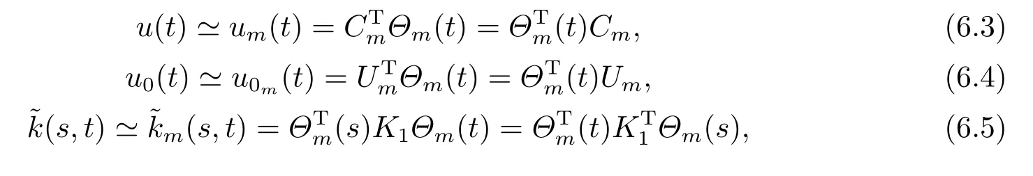
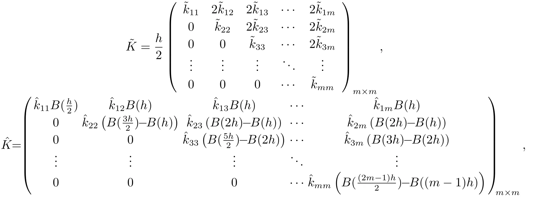
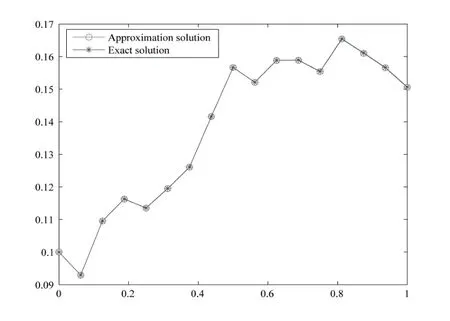
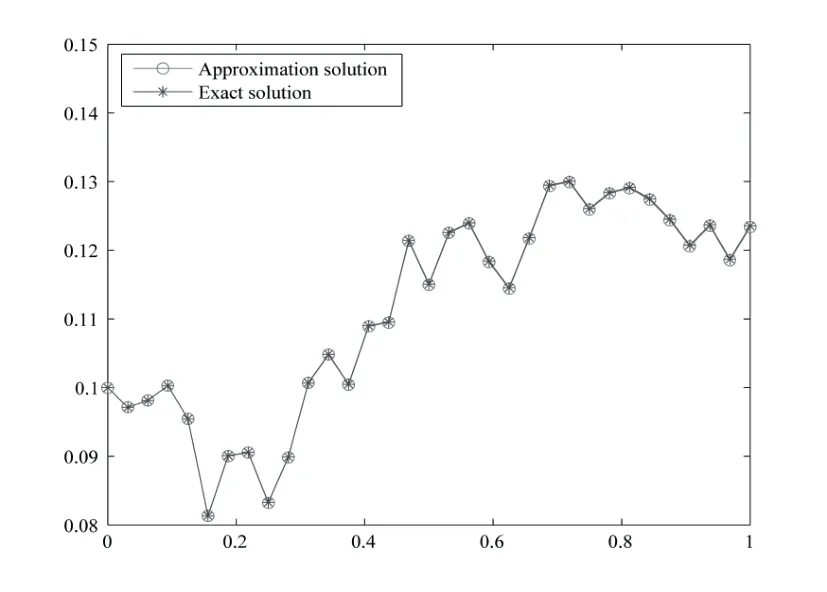
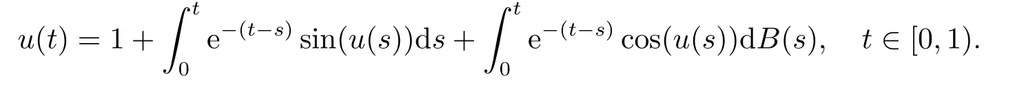
Whent=We can sett?(i?1)h ?,for (i?1)h≤t

where theith element is

Therefore

where the integration operational matrix is given by

Thus,every integral functionu(t) can be approximated as follows

4.Stochastic Integration Operational Matrix

Therefore

where the stochastic integration operational matrix is given by

5.Error Analysis

In this section,we prove that the approximate solution is convergent of orderO(h),Firstly,we recall two useful lemmas.

Lemma 5.1[6,15]Letv(s) be an arbitrary bounded function on [0,1) and(s)=v(s)?vm(s),wherevm(s) is the approximation of BPFs ofv(s),then

Lemma 5.2[6,15]Letv(x,y)be an arbitrary bounded function onD=[0,1)×[0,1)andêm(x,y)=v(x,y)?vm(x,y),wherevm(x,y) is the approximations of BPFs ofv(x,y),then

Secondly,letem(t)=u(t)?um(t),whereum(t)is the approximate solution ofu(t)defined in (1.3),u0m(t),(s,t) and(s,t) respectively are approximations of BPFs ofu0(t),(s,t)and(s,t).

The following is the main convergence theorem.

Theorem 5.1Supposeσandgare bounded analytic functions and satisfy the Lipschitz conditions:

(i′)|σ(x)?σ(y)|≤l1|(x?y)|,|g(x)?g(y)|≤l3|(x?y)|;

(ii′)|σ(x)|≤l2,|g(x)|≤l4;

(iii′)|(s,t)|≤l5,|(s,t)|≤l6,li,i=1,2,···,6 are positive constants.Then,

ProofFor (5.3),we have

Then,we can get

or

By Gronwall’s inequality,we have

Then,

By using (5.1)(5.2),we have

The last equation can be converted into

wherepi,i=1,2,···,6 are independent nonnegative constants.The proof is completed.

6.Numerical Method

In this section,we apply BPFs to solve nonlinear stochastic It?-Volterra integral equation(1.3),whereu0(t) is known function,(s,t) and(s,t) are kernel functions defined on 0

Lemma 6.1Letbe the analytic functions for positive integerj∈(0,∞),then

whereΘm(t) andCmare derived in (2.3) and (2.4),

ProofBy virtue of the known conditions and the disjointness of BPFs defined in(2.1),we can get

Thus,

The proof is completed.

Now,in order to solve Equation (1.3),we supposeu(t),u0(t),(s,t) and(s,t) could be approximated in terms of BPFs as follows

whereCmandUmare block pulse coefficient vectors,K1andK2are block pulse coefficient matrices similar to (2.5).Substituting the above approximations (6.1)-(6.6) into Equation(1.3),we have

Applying the operational matricesQmandfor BPFs derived in (3.1) and (4.1),we have

For this nonlinear equation (6.7),there are various methods to solve its numerical solution,such as simple trapezoid method,Simpson method and Romberg method,which are often introduced in the numerical analysis course.In this paper,we will use the int()function provided by Matlab to solve the nonlinear equation set[3].

7.Numerical Results and Discussion

In the last section,we consider the following two examples which illustrate the method is efficient.

Example 7.1Consider the following nonlinear stochastic integral equation

the exact solution of the above equation is

This equation has been given in[2,14].In[2],the numerical solution was obtained by hat function.However,simpler BPFs is used in this article,and the error means in the following tables illustrate that our accuracy is not lower than or even higher than those in [2].

Fig.1 m=16,simulation results of approximate solution and exact solution for Example 7.1

Fig.2 m=32,simulation results of approximate solution and exact solution for Example 7.1

The exact and approximate solutions of the Example 7.1 form=16 andm=32 are respectively given in Fig.1 and Fig.2.

The error meansM,error standard deviationsSand confidence intervals for error means of Example 7.1 form=16 andm=32 are respectively given in Tab.1 and Tab.2.

Tab.1 Whenm=16,this table shows error means M, error standard deviations S and confidence intervals for different time t

Tab.2 Whenm=32,this table shows error means M, error standard deviations S and confidence intervals for different time t

From the above figures and tables,the errors between the exact solutions and approximate solutions are very small.This method is effective to solve the low-dimensional stochastic It?-Volterra integral equations.However,for high-dimensional stochastic It-Volterra integral equations,the calculation amount of this method increases obviously.

Example 7.2Consider the following nonlinear stochastic It-Volterra integral equation(for details,see [19])

The mean and approximate solutions of Example 7.2 form=16 andm=32 are respectively given in Fig.3 and Fig.4.

Fig.3 m=16,simulation results of approximate solution and mean solution for Example 7.2

Fig.4 m=32,simulation results of approximate solution and mean solution for Example 7.2

This example shows a comparison of the approximate solutions and the mean solutions.From the figures,we find the approximate solutions fluctuate around the mean orbit.Whateverm=16 orm=32,the general trends of the mean solutions are similar.

8.Conclusion

For some stochastic Volterra integral equations,exact solutions can not be found.But,the numerical solution can be conveniently determined based on stochastic numerical analysis.A variety of methods for solving linear stochastic Volterra integral equation have been given.As the complexity of the system,we use BPFs as the basis function to solve the nonlinear stochastic Volterra integral equation.It is simple and effective.