
UNIQUENESS OF THE INVERSE TRANSMISSION SCATTERING WITH A CONDUCTIVE BOUNDARY CONDITION?
2021-06-17 13:59:50向建立嚴(yán)國政
關(guān)鍵詞:國政
(向建立) (嚴(yán)國政)
School of Mathematics and Statistics,Central China Normal University,Wuhan 430079,China
E-mail:xiangjl@mails.ccnu.edu.cn;yangz@mail.ccnu.edu.cn
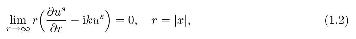
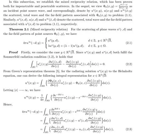
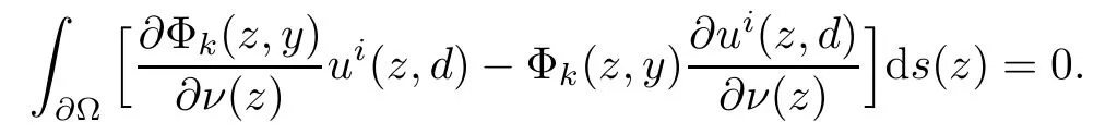
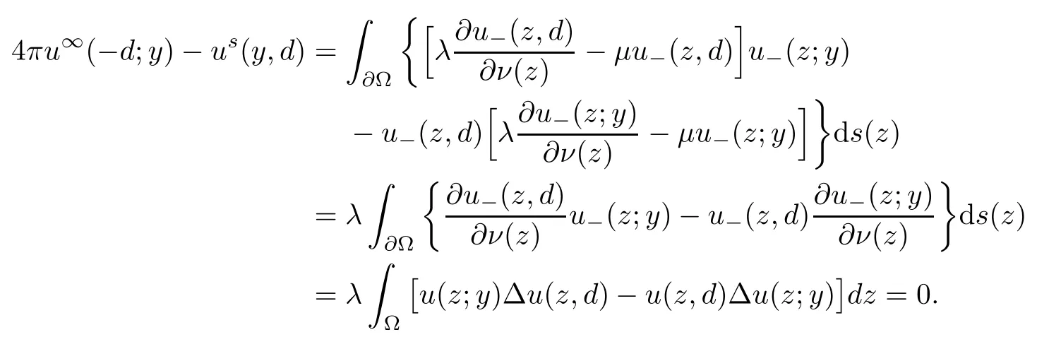
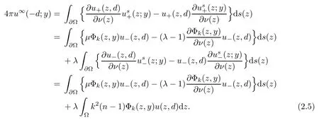
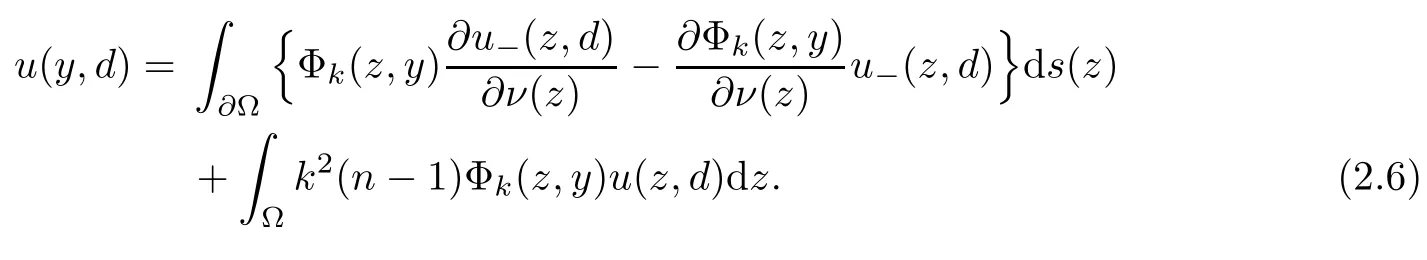
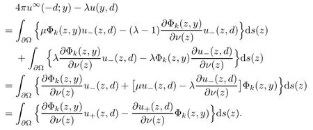
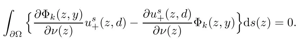
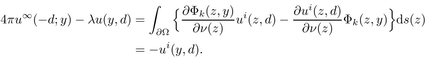
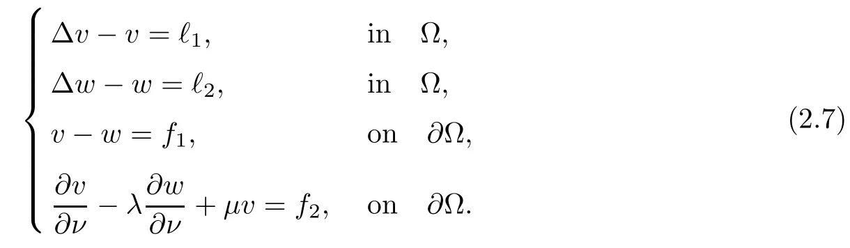
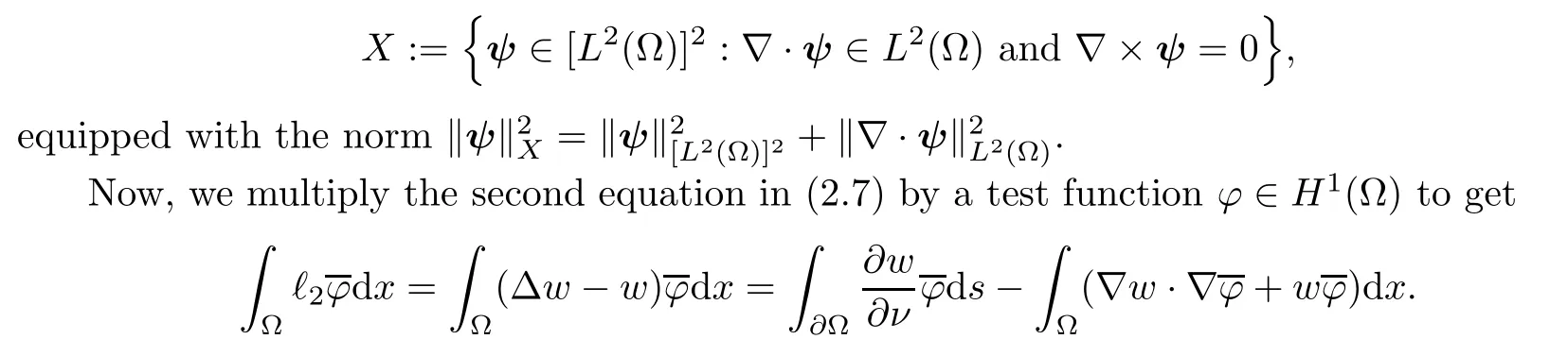
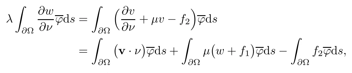
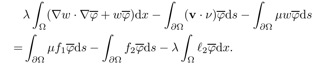
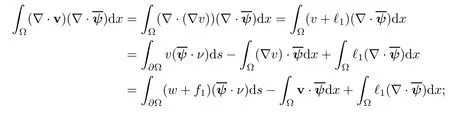
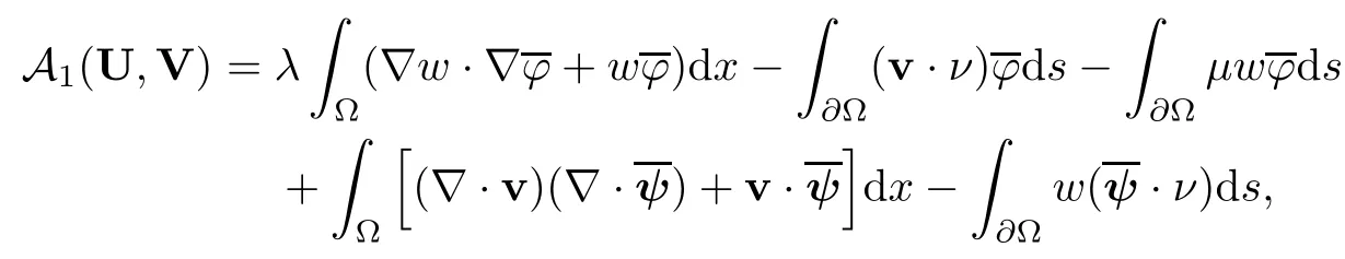
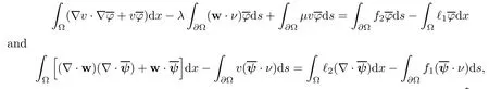
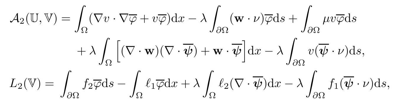
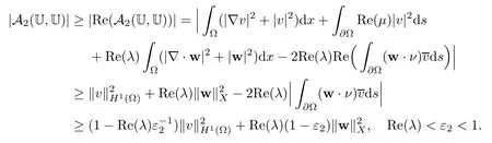
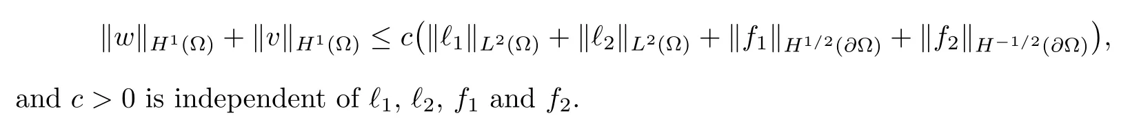
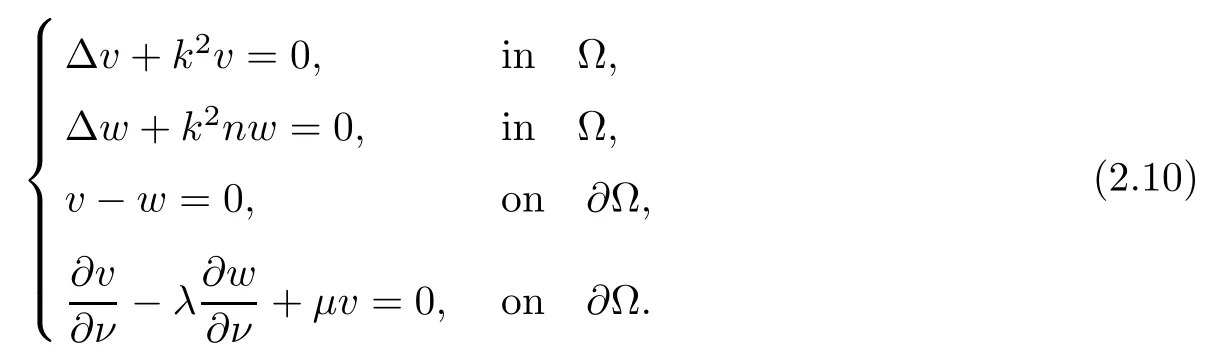
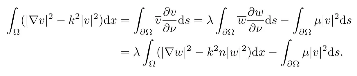
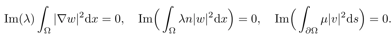
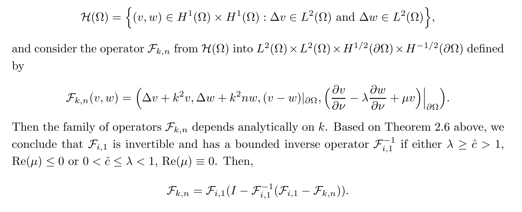
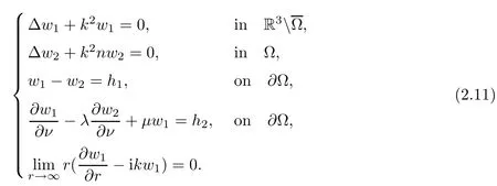
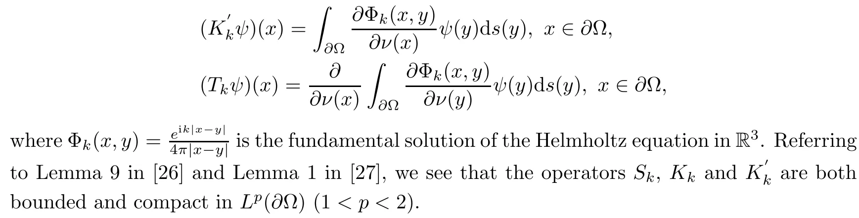
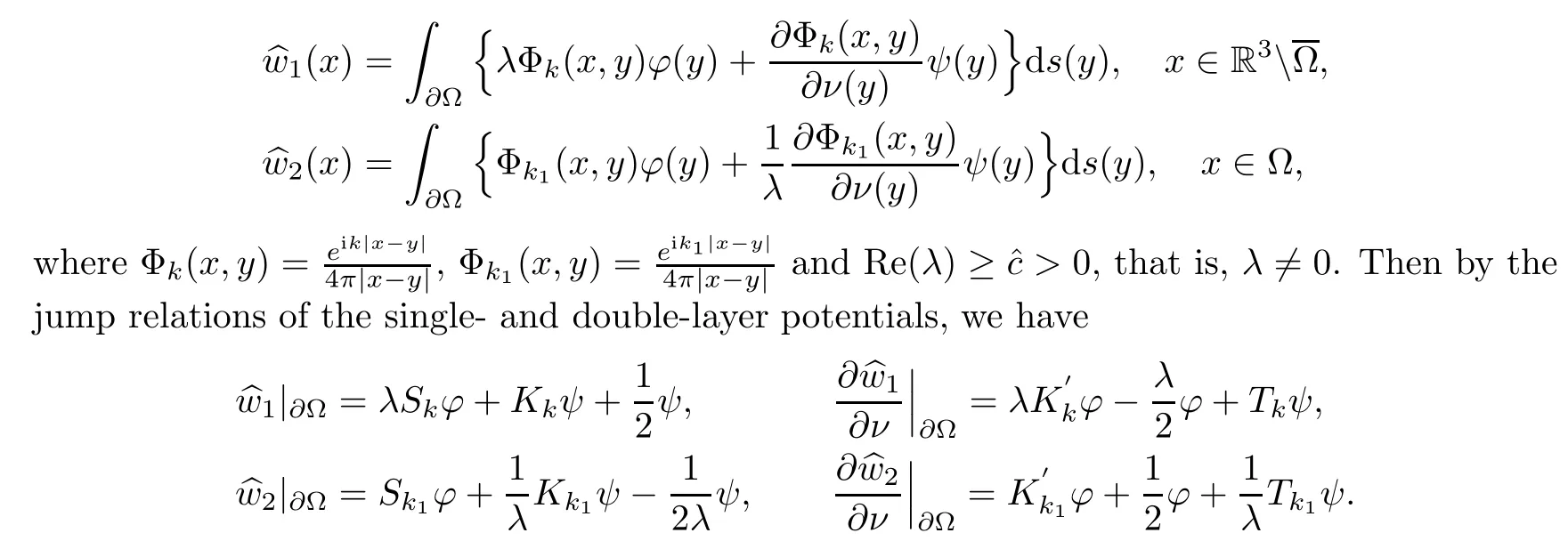
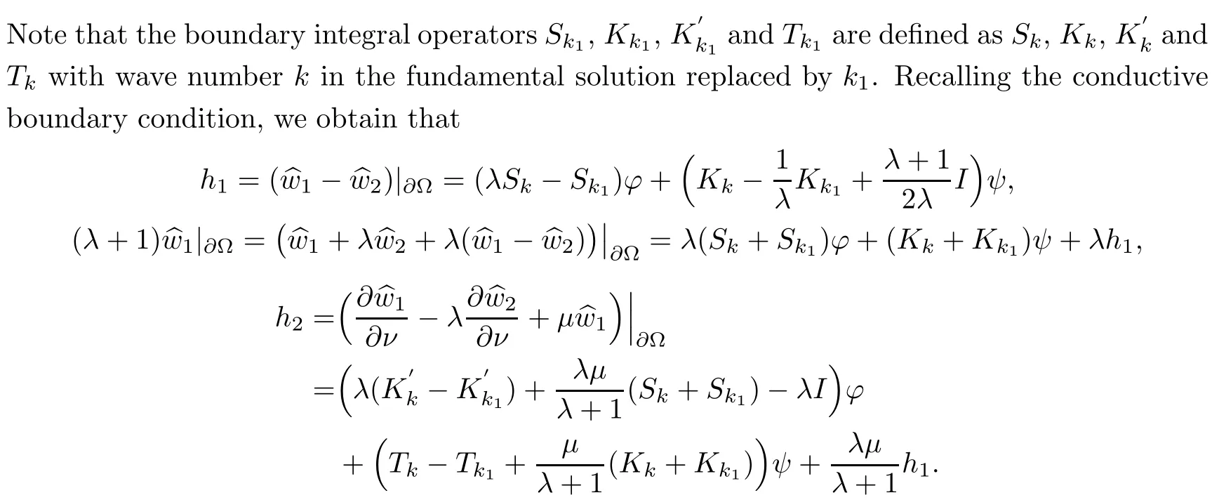
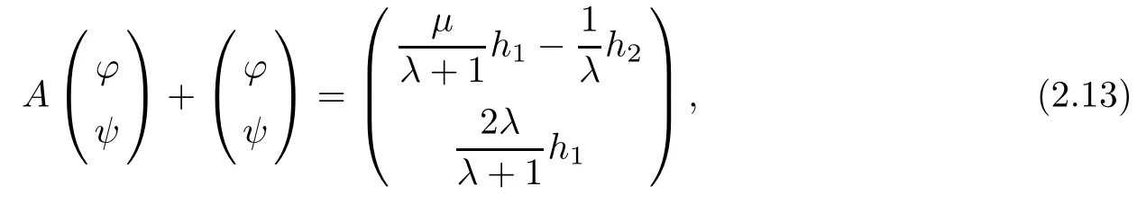
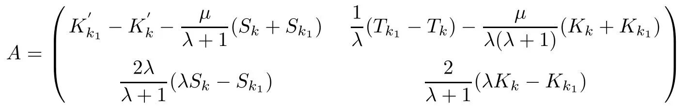
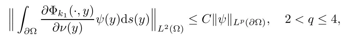
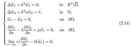
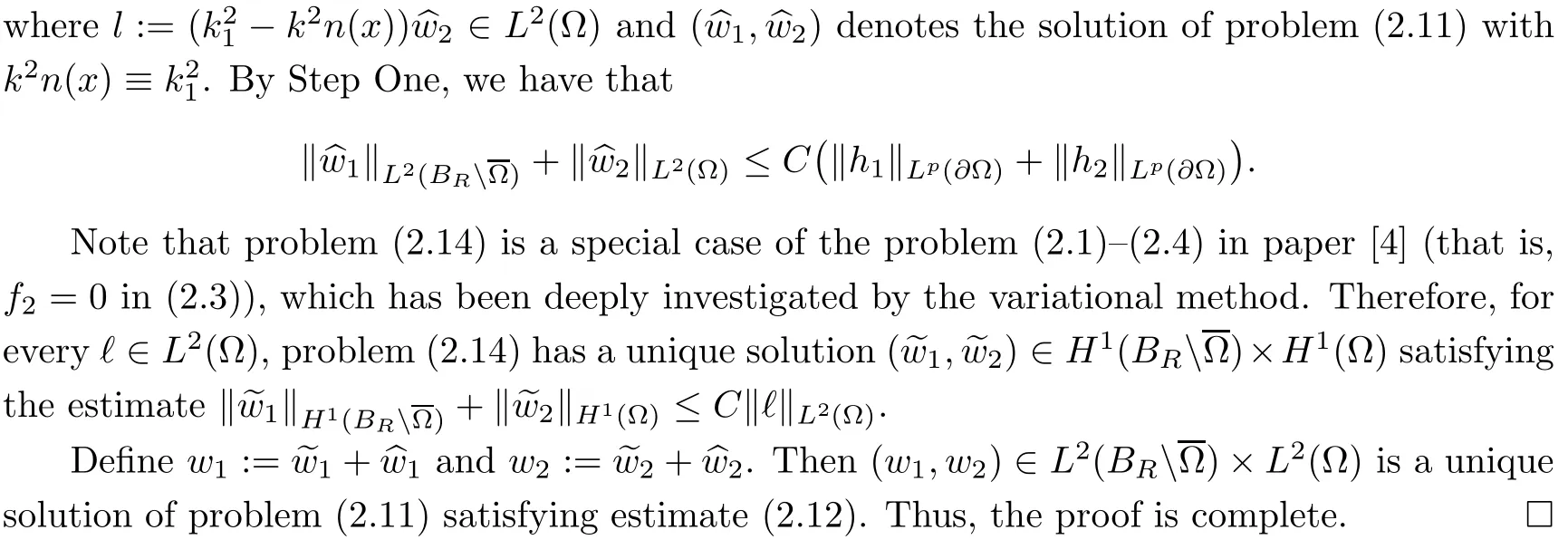
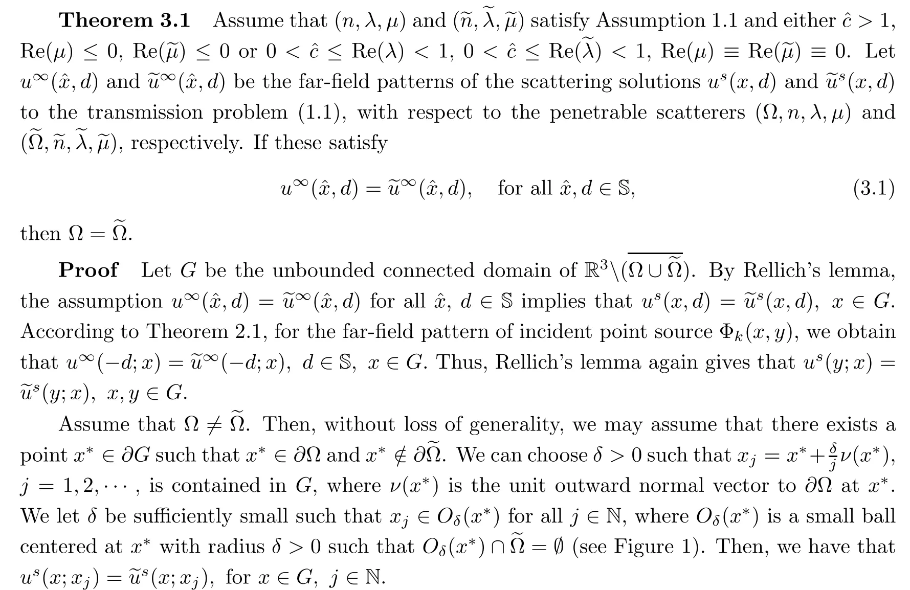
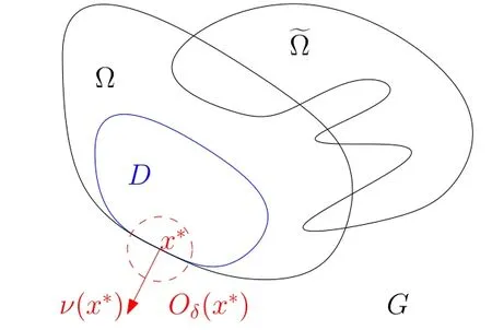
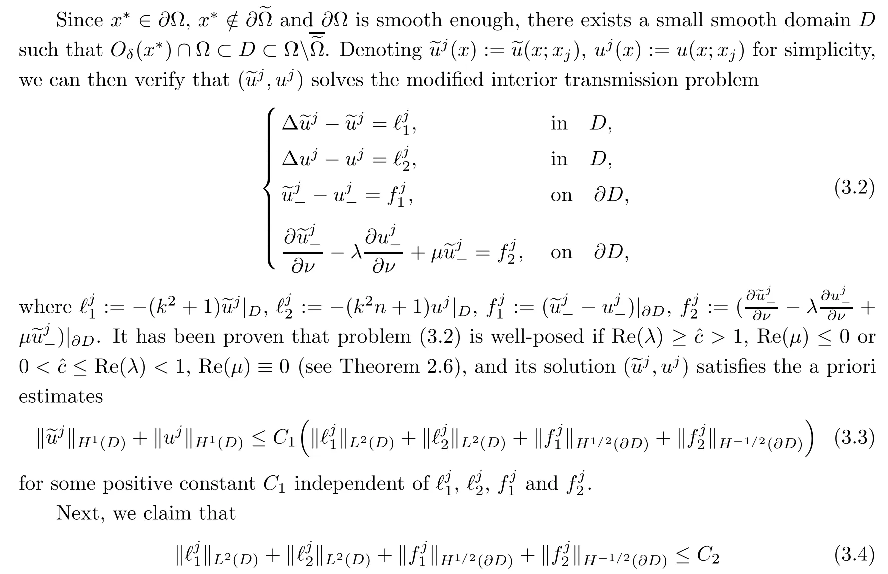
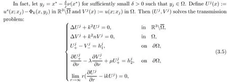
Abstract This paper considers the inverse acoustic wave scattering by a bounded penetrable obstacle with a conductive boundary condition.We will show that the penetrable scatterer can be uniquely determined by its far-field pattern of the scattered field for all incident plane waves at a fixed wave number.In the first part of this paper,adequate preparations for the main uniqueness result are made.We establish the mixed reciprocity relation between the far-field pattern corresponding to point sources and the scattered field corresponding to plane waves.Then the well-posedness of a modified interior transmission problem is deeply investigated by the variational method.Finally,the a priori estimates of solutions to the general transmission problem with boundary data in Lp(?Ω)(1 Key words Acoustic wave;uniqueness;mixed reciprocity relation;modified interior transmission problem;a priori estimates The inverse scattering problem we are concerned with here is determining the shape of an obstacle by measurements of the far-field patterns of acoustic waves.We are interested in the scattering of a penetrable obstacle covered by a thin layer of high conductivity;that is,the so-called conductive boundary condition([1,2]),which is a generalization of the classical transmission problem. Let ? denote a penetrable bounded open domain in R3withconnected.Let n(x)be the refractive index,let k>0 be the wave number,and set a jump parameter λ∈C{0}and a complex-valued functionμon the smooth boundary??.Then the conductive scattering problem we consider is modeled as follows: where u=ui+usis the total field,which is a superposition of the incident wave ui=ui(x,d):=eikx·d(note that the incident wave will be a plane wave or a point source in our later proofs and that d denotes the incident direction)and the scattered wave us,and ν is the unit outward normal to the boundary??.Here,u±anddenote the limit of u andfrom the exterior(+)and interior(?),respectively.Furthermore,the scattered field ussatisfies the Sommerfeld radiation condition and the convergence holds uniformly with respect to=x/|x|∈S,where S denotes the unit sphere in R3. Referring to Section 2 of paper[4],we make following assumptions on n,λ andμto guarantee the well-posedness of the direct problem(1.1): Assumption 1.1(1)The refractive function n∈L∞(?)satisfies Re(n)>0 and Im(n)≥0 almost everywhere(a.e.)in ?. (2)λ is a non-zero complex constant,such that there exists>0,such that Re(λ)≥and Im(λ)≤0,Im(λn)≥0 a.e.in ?. (3)μ∈L∞(??)with Re(μ)≤0 and Im(μ)≥0 a.e.on??. It is well known that the radiating solution ushas the asymptotic expansion uniformly for all directions=x/|x|∈S.Here,u∞is called the far-field pattern of us,which is an analytic function defined on S. The problem of uniqueness in the inverse obstacle scattering theory is of central importance both for the theoretical study and the implementation of numerical algorithms in acoustic,electromagnetic,fluid-solid interaction and elastic waves,etc..The first uniqueness result was shown by Schiffer[20]in acoustic waves with a Dirichlet boundary condition whose argument cannot be transferred to other boundary conditions.In 1990,Isakov[17]gave a uniqueness proof for transmission problems(ui=ue,?ue/?ν=μ?ui/?ν,μ/=1)based on the variational method by constructing a sequence of singular solutions.In 1993,Kirsch and Kress[18]simplified Isakov’s proof and also transferred it to the Neumann boundary condition by proving a continuous dependence result in a weighted Banach space of continuous functions.In the same year,Ramm[31]used a new method to prove the uniqueness of the impenetrable obstacle with a Dirichlet or Neumann boundary condition. In 1994,Hettlich[16]achieved the uniqueness theorem for the general conductive boundary condition(u+?u?=0,?u+/?ν?μ?u?/?ν=λu,the interior wave number is a constant)based on the idea of Isakov.Furthermore,the uniqueness of coefficientsμ,λ and the constant interior wave number were also proven.Later,in 1996,Gerlach and Kress[12]simplified and shortened the analysis of Hettlich.In order to present a refinement in the case when the boundary of the scatterer is allowed to have irregularities,in 1998,Mitrea[24]studied its uniqueness dependent upon boundary integral techniques and the Calderón-Zygmund theory.In 2004,Valdivia[33]worked on the uniqueness again based on the original idea of Isakov.Since then,there have been many other uniqueness problems,such as impenetrable scatterers with an unknown type of boundary condition([10,19]),local uniqueness([13,32]),penetrable orthotropic[11]or anisotropic inhomogeneous obstacles([14,25]),a piecewise homogeneous medium([21–23]),etc.. In this paper,we again consider the uniqueness of the inverse transmission scattering with a conductive boundary condition by an inhomogeneous medium.The idea is inspired by[29](an inhomogeneous acoustic cavity),[30](fluid-solid interaction with embedded obstacles)and[34](penetrable obstacles with embedded objects in acoustic and electromagnetic scattering).Hence,before showing the main uniqueness proof,we discuss some important preparations,which are also of interest in their own right. Firstly,we establish a mixed reciprocity relation between the far-field pattern corresponding to point sources and the scattered field corresponding to plane waves of this general transmission problem.The mixed reciprocity relation was shown in[26](Theorem1)for sound-soft and sound-hard obstacles,in[9](Theorem 3.24)for generalized impedance objects,in[28](Theorem 2.2.4)for inhomogeneous media,and in[23]for a piecewise homogeneous medium,etc..In the derivation of(2.1)and the above references,we can conclude that the relation for y∈R3? is valid for all possible boundary conditions of penetrable or impenetrable scatterers.Furthermore,for y∈?,relation(2.1)has a close connection with the jump parameter λ(Lemma 3.2 in[23]),but that disregards the complex-valued functionμ. Secondly,we study the well-posedness of a modified interior transmission problem by the variational method.Though the interior transmission problems have been deeply investigated in the book[6],there are few results about the conductive boundary([3,15]for λ=1).The well-posedness is achieved under some limitations on λ andμ,and the discreteness of interior transmission eigenvalues is a by-product.In the future,we want to conduct further research on the interior transmission eigenvalues problem. Thirdly,we prove the a priori estimates of solutions to the general transmission problem with boundary data in Lp(??)(1 Finally,the novel and simple method for proving the uniqueness of the conductive boundary by its far field pattern is easy to implement for our inverse transmission problem. The remainder section of the paper is organized as follows:Section 2 is devoted to making preparations;we show a mixed reciprocity relation,investigate the well-posedness of a modified interior transmission problem,and construct the a priori estimates of solutions to the general transmission problem with boundary data in Lp(??)(1 In this section,we make some necessary preparations before showing the uniqueness of the inverse problem(1.1). where the last equality is obtained by adding formula(2.2). Using Green’s representation theorem again,for y∈ Applying Green’s second integral theorem to ui(·,d)and Φk(·,y)in ? yields Adding up the previous two equalities,we arrive at Combining(2.3)with(2.4),we find that Use the conductive boundary condition and Green’s formula in ?,we conclude that This implies that 4πu∞(?d;y)=us(y,d)for all d∈S,y∈ Secondly,we consider the case y∈?.Recalling equality(2.3),which holds also for y∈?,using the conductive boundary condition,we obtain The last equality is obtained completely similar to the proof of(3.13)to(3.14)in Lemma 3.2([23]). On the other hand,with the help of Green’s representation formula,we know that Combining(2.5)with(2.6)and using the conductive boundary condition,we have For y∈?,both Φk(·,y)and us(·,d)satisfy the Helmholtz equation inand the Sommerfeld radiation condition(1.2),hence Consequently, This implies that 4πu∞(?d;y)=λus(y,d)+(λ?1)ui(y,d)for all d∈S,y∈?.The proof is complete. □ Remark 2.2If there is a buried object inside ?,Theorem 2.1 also holds.Lemma 3.2 in[23]is a special case when n is a constant andμ=0 a.e.on??. Remark 2.3Theorem 2.1 also holds in two dimensional space with some modifications of the coefficient. Given ?1,?2∈L2(?),f1∈H1/2(??),f2∈H?1/2(??),we consider the following modified interior transmission problem: In order to reformulate(2.7)as an equivalent variational problem,we define the Hilbert space Using the conductive boundary condition in(2.7),we see that wherev=?v,and thenv∈X.After arranging,we obtain that We multiply the first equation in(2.7)by a test function ψ∈X.Similarly,integrating in ?and using the boundary condition,we obtain that is Based on the above calculations,we introduce the sesquilinear form A1(U,V),defined on{H1(?)×X}2by whereU:=(w,v)andV:=(?,ψ)are in H1(?)×X.We denote by L1:H1(?)×X?→C the bounded antilinear functional given by Therefore,the variational formulation of problem(2.7)is to findU=(w,v)∈H1(?)×X such that Changing the roles of w and v,we can obtain another different variational formulation of problem(2.7);namely,we multiply the first equation in(2.7)by a test function ?∈H1(?)and the second equation by a test function ψ∈X,integrate in ?,and use the boundary condition to obtain wherew=?w,and thenw∈X. We introduce the sesquilinear form A2(U,V)defined on{H1(?)×X}2and the bounded antilinear functional L2:H1(?)×X?→C given by where U:=(v,w)and V:=(?,ψ)are in H1(?)×X.Then,the variational formulation of problem(2.7)is to find U=(v,w)∈H1(?)×X such that The following Theorem states the equivalence between problems(2.7)and(2.8)or(2.9)(the detailed proof is the same as that of Theorem 3.3 in the paper[7]and Theorem 6.5 in the book[5],so for brevity we omit it here): Theorem 2.4Problem(2.7)has a unique solution(w,v)∈H1(?)×H1(?)if and only if problem(2.8)has a unique solutionU=(w,v)∈H1(?)×X or problem(2.9)has a unique solution U=(v,w)∈H1(?)×X. Now,we investigate the modified interior transmission problem in the variational formulations(2.8)and(2.9). Theorem 2.5(1)If Re(λ)≥>1 and Re(μ)≤0,then the variational problem(2.8)has a unique solutionU=(w,v)∈H1(?)×X that satisfies where cj>0(j=1,2)is independent of ?1,?2,f1and f2. ProofThe trace theorems and Schwarz’s inequality ensure the continuity of the antilinear functional Lj(j=1,2)on H1(?)×X and the existence of a constant cjwhich is independent of ?1,?2,f1and f2such that For the first part,ifU=(w,v)∈H1(?)×X,the assumptions that Re(λ)≥>1 and Re(μ)≤0 imply that For the second part,if U=(v,w)∈H1(?)×X,the assumptions that 0<≤Re(λ)<1 and Re(μ)≡0 imply that Hence Aj(j=1,2)is coercive.The continuity of Ajfollows easily from Schwarz’s inequality and the classical trace theorems.Then Theorem 2.5 is a direct consequence of the Lax-Milgram Lemma applied to(2.8)and(2.9). □ Combining the above two Theorems 2.4 and 2.5,we obtain the well-posedness of the modified interior transmission problem(2.7). Theorem 2.6Assume that Re(λ)≥>1,Re(μ)≤0 or 0<≤Re(λ)<1,Re(μ)≡0.Then the modified interior transmission problem(2.7)has a unique solution(w,v)∈H1(?)×H1(?)that satisfies Using the analytic Fredholm theory(see Section 8.5 in the book[9]),we get a by-product regarding the discreteness of the following interior transmission eigenvalues problem: Definition 2.7Values of k for which the above interior transmission problem(2.10)has a nontrivial solution pair(v,w)∈H1(?)×H1(?)are called transmission eigenvalues. Before we establish the discreteness result,we first study the case when there are no real transmission eigenvalues. Lemma 2.8Assume that n,λ andμsatisfy Assumption 1.1.If either Im(λ)<0 or Im(n)>0 almost everywhere in ?,then there are no real transmission eigenvalues of the problem(2.10). ProofLet v and w be a solution pair of the interior transmission problem(2.10).Applying Green’s identity to v and w,we have Since Im(μ)≥0,Im(λ)≤0,Im(λn)≥0,we have that If Im(λ)<0 a.e.in ?,then?w=0 in ?,from the equation w=0.From the boundary condition in(2.10)and the integral representation formula,v also vanishes in ?. If Im(λ)=0 and Im(n)>0 a.e.in ?,then λ≥>0 and Im(λn)=λIm(n)>0.Hence,w=0 and v=0 in ?.This completes the proof. □ Remark 2.9From the proof of Lemma 2.8,we conclude that k may be an interior transmission eigenvalue of(2.10)if Im(λ)=0 and Im(n)=0.In this case,if Im(μ)>0 almost everywhere on??,we further obtain that v=0 on??,whence the eigenvalues of(2.10)form a subset of the classical Dirichlet eigenvalues of?Δ in ?. Theorem 2.10Assume that n,λ andμsatisfy Assumption 1.1 and that Im(λ)=0 and Im(n)=0.If either λ≥>1,Re(μ)≤0 or 0<≤λ<1,Re(μ)≡0,then the transmission eigenvalues of(2.10)form a discrete(possibly empty)set with+∞as the only possible accumulation point. ProofLet us set Since(Fi,1?Fk,n)(w,v)=(?(1+k2)v,?(1+k2n)w,0,0)is compact based on the compact embedding of H1(?)to L2(?),we conclude that the transmission eigenvalues form a discrete(possibly empty)set with+∞as the only possible accumulation point by the analytic Fredholm theory(Section 8.5 of the book[9]).The proof is complete. □ Remark 2.11For the case λ=1,the discreteness and existence of the transmission eigenvalues have been proven clearly in[3]. By employing the boundary integral equation method([8,27,34]),we establish the a priori estimates of the solution to the following general transmission problem(2.11)with boundary data in Lp(??)(1 We introduce the single-and double-layer boundary integral operators and their normal derivative operators Theorem 2.12Assuming that n,λ andμsatisfy Assumption 1.1.For h1,h2∈Lp(??)with 4/3≤p<2,the transmission problem(2.11)has a unique solution pair(w1,w2)∈satisfying that where BRdenotes a large ball centered at the origin with radius R such thatand C is a positive constant depending on R. ProofIn order to apply the boundary integral equation method,we divide our proof into two steps(refer to Theorem 2.5 in[34]). Step OneAssume that k2n(x)≡>0 is a constant.We seek a solution pairof problem(2.11)in the following form: Here,I denotes the identity operator.Then the transmission problem(2.11)can be reduced to a system of the integral equations where the integral matrix operator A is given by Since all elements of A are compact operators in the corresponding Banach spaces,it is easy to see that A+I(I denotes the identity matrix)is a Fredholm operator with index zero.Together with the uniqueness of the direct transmission problem(2.11),there exists a unique solution(?,ψ)∈Lp(??)×Lp(??)of system(2.13)satisfying the estimate Referring to inequalities(2.22)and(2.23)in the paper[34](Theorem 2.5),that is, where 1/p+1/q=1 and we achieve estimate(2.12). Step TwoFor the general case n(x)∈L∞(?),we consider the following problem: In this section,we consider the uniqueness of the inverse transmission problem(1.1).Under some restrictions on λ andμ,we use a simple and novel method to show that the penetrable obstacle can be uniquely determined by its far-field pattern associated with plane waves. Figure 1 Possible choice of x? uniformly for all j∈N,where C2>0 is independent of j. where Remark 3.2If there are impenetrable buried objects inside ?,the penetrable obstacle can also be uniquely determined by our method,with small modifications in subsections 2.1(Remark 2.2)and 2.3(Theorem 2.5 in[34]).Furthermore,the buried object will be determined by the mixed reciprocity relation(2.1),after discovering the penetrable surface(Theorem 3.7 in[23]).1 Introduction

2 Preparations
2.1 Mixed reciprocity relation

2.2 Modified interior transmission problem


2.3 A priori estimates for the transmission problem with Lp data


3 Uniqueness of the Inverse Transmission Problem
 猜你喜歡
新傳奇(2021年18期)2021-05-21 08:34:10環(huán)球時報(2019-07-23)2019-07-23 06:16:14資源導(dǎo)刊(2016年4期)2016-07-12 10:01:33學(xué)苑創(chuàng)造·A版(2016年7期)2016-07-06 06:03:07資源導(dǎo)刊(2015年6期)2015-02-01 01:50:11環(huán)球時報(2015-01-14)2015-01-14 22:50:54黨史文匯(2013年2期)2013-02-20 06:45:10
猜你喜歡
新傳奇(2021年18期)2021-05-21 08:34:10環(huán)球時報(2019-07-23)2019-07-23 06:16:14資源導(dǎo)刊(2016年4期)2016-07-12 10:01:33學(xué)苑創(chuàng)造·A版(2016年7期)2016-07-06 06:03:07資源導(dǎo)刊(2015年6期)2015-02-01 01:50:11環(huán)球時報(2015-01-14)2015-01-14 22:50:54黨史文匯(2013年2期)2013-02-20 06:45:10
 Acta Mathematica Scientia(English Series)2021年3期