
DYNAMICS ANALYSIS OF A DELAYED HIV INFECTION MODEL WITH CTL IMMUNE RESPONSE AND ANTIBODY IMMUNE RESPONSE?
2021-06-17 14:00:04楊俊仙
關(guān)鍵詞:楊俊
(楊俊仙)
School of Science,Anhui Agricultural University,Hefei 230036,China
E-mail:yangjunxian1976@126.com
Leihong WANG(王雷宏)
School of Forestry and Landscape Architecture,Anhui Agricultural University,Hefei 230036,China
E-mail:wangleihong208010@126.com
Abstract In this paper,dynamics analysis of a delayed HIV infection model with CTL immune response and antibody immune response is investigated.The model involves the concentrations of uninfected cells,infected cells,free virus,CTL response cells,and antibody antibody response cells.There are three delays in the model:the intracellular delay,virus replication delay and the antibody delay.The basic reproductive number of viral infection,the antibody immune reproductive number,the CTL immune reproductive number,the CTL immune competitive reproductive number and the antibody immune competitive reproductive number are derived.By means of Lyapunov functionals and LaSalle’s invariance principle,sufficient conditions for the stability of each equilibrium is established.The results show that the intracellular delay and virus replication delay do not impact upon the stability of each equilibrium,but when the antibody delay is positive,Hopf bifurcation at the antibody response and the interior equilibrium will exist by using the antibody delay as a bifurcation parameter.Numerical simulations are carried out to justify the analytical results.
Key words Beddington-DeAngelis incidence;CTL immune response;antibody immune response;delay
1 Introduction
As is well known,Human Immunodeficiency Virus(HIV)and Acquired Immune Deficiency Syndrome(AIDS)are a serious threat to human health.The main target of HIV/AIDS is CD4+T cells–which is one type of white blood cell in the human immune system–and it can cause the number of CD4+T cells to decrease greatly.HIV seriously affects the ability of patients to defend opportunistic infections,so the eradication of HIV is the ultimate goal of research groups worldwide.Mathematical models are of great significance in terms of understanding the dynamics of populations in the context of epidemics.Models of virus infection in the host have been widely studied,and have provided insight into the dynamics of viral load in vivo for further research on the progress and control of HIV[1–30].In particular,issues including stability and Hopf bifurcation provide specific information for us to be able to understand disease control.
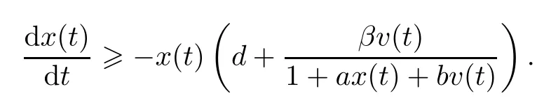
It should be pointed out that immune response during the process of viral infection is universal and necessary to eliminate or control the disease.The models which include the adaptive immune response in fighting free viruses and in reducing the number of infected cells have been studied[3–5].This adaptive immunity is represented by Cytotoxic T Lymphocyte(CTL)and antibody immune responses.CTL immune response cells,which attack infected cells,play a critical part in defending against HIV.Hence,viral infection models with CTL immune response cells have received much attention[9–13,16–20,22,26,29,30].Recently,scientists have discovered that some patients produce a potent immune molecule,called a broadly neutralizing antibody,which recognizes many different HIV viruses[14,15].An effective immune system needs both the antibody and CTL immune responses to prevent HIV infection.Thus,the HIV infection model that incorporates both the antibody and CTL immune responses could be a realistic model for describing the dynamics of HIV infection[16–20,29,30].In[16],a basic model with bilinear incidence was proposed to describe the interactions of the antibody and CTL immune responses,and it included uninfected target cells x(t),productively infected cells y(t),free virus v(t),CTL immune response cells z(t)and antibody response cells w(t).It was assumed that the incidence rate is bilinear in the model,namely,that the infection rate per host and per virus is a constant,but experiments have shown that the incident rate is probably not linear over the entire interaction range of susceptible cells x(t)and virus v(t)[6,7,10,19–30].In[22–29],a more general infection rate,the Beddington-DeAngelis incidence ratewas proposed,where a and b are positive constants.In[29],Miao et al.investigated the HIV infection model with a Beddington-DeAngelis functional response and three delays:the intracellular delay,virus replication delay,and immune response delay.They reached the conclusion that the intracellular delay and virus replication delay do not affect the stability of the equilibria,but that the immune response delay markedly affects the stability of CTL response equilibrium and the interior equilibrium.In[30],Guo et al.pointed out the antibody delay cannot be ignored in the viral infection model.This raises the question:how will the antibody delay affect the equilibrium of system(1.1)?This will be the focus of our consideration.
In this paper,we consider a five-dimensional HIV infection model with a Beddington-DeAngelis incidence rate and three time delays describing the intracellular delay,the virus replication delay,and the antibody delay as follows:

Here,Λ,k,c and g are the proliferation rate of the uninfected cells,the virus,the CTL response cells and the antibody response cells,respectively;β is the infection rate constant;d,r,u,h and α represent the death rate constants of uninfected target cells,productively infected cells,virus,CTL response cells and antibody response cells,respectively;p represents the killing rate of infected cells by CTL response cells;q is the antibody cells neutralization rate;τ1denotes the intracellular delay anddenotes the surviving rate of infected cells during delay period[t?τ1,t];τ2is the virus replication delay,denotes the surviving rate of the virus during the delay period[t?τ2,t],τ3denotes the antibody response delay.
Let τ=max{τ1,τ2,τ3}and={(x1,x2,x3,x4,x5):xi≥0,i=1,2,3,4,5},C([?τ,0],)denote the space of continuous functions mapping the interval[?τ,0]into.The initial condition for system(1.1)is

where(φ1(θ),φ2(θ),φ3(θ),φ4(θ),φ5(θ))∈C([?τ,0],).It is well known,by the fundamental theory of functional differential equations(see[31]),that system(1.1)has a unique solution(x(t),y(t),v(t),z(t),w(t))satisfying the initial conditions(1.2).
The organization of this paper is as follows:in the next section,the basic properties of model(1.1)for the boundedness of solutions,the threshold values and the existence of five equilibria are discussed.In Section 3,the threshold conditions on the global stability and instability for the infection-free equilibrium E0,immune-free equilibrium E1and infection equilibrium E3with only CTL immune responses are stated.When τ3=0,the threshold conditions on the global stability and instability for the infection equilibrium E2with only antibody responses and infection equilibrium E4with both CTL immune responses and antibody responses are proved.In Section 4,when τ3>0,the sufficient conditions on the existence of Hopf bifurcation for the infection equilibrium E2with only antibody responses and infection equilibrium E4with both CTL and antibody responses are established.In Section 5,the numerical simulations are carried out to further illustrate the dynamical behaviour of the model.Finally,we will give a discussion.
2 Preliminaries
In this section,we discuss the basic properties of model(1.1)for the non-negativity and boundedness of solutions,the threshold values and the existence of five equilibria.
2.1 Non-negativity and Boundedness of solutions
Theorem 2.1Let(x(t),y(t),v(t),z(t),w(t))be the solution of model(1.1)satisfying initial conditions(1.2).Then x(t),y(t),v(t),z(t)and w(t)are nonnegative and bounded on[0,+∞).
ProofFrom(1.1),we know that,for t≥0,
This implies that

In a similar way,we obtain that z(t)>0 and w(t)>0.
Using Lemma 2 from the work of Yang et al.[32],we obtain that y(t)>0 and v(t)>0.
Next,we establish the boundedness of the solutions of system(1.1).Define

We have
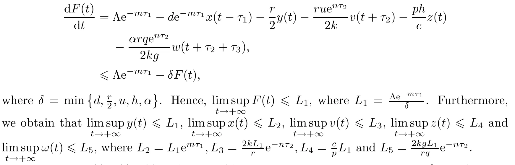
Therefore,x(t),y(t),v(t),z(t)and w(t)are nonnegative and bounded on[0,+∞).This completes the proof. □
2.2 The existence of equilibria
Clearly,system(1.1)always exists an infection-free equilibrium E0(x0,0,0,0,0),where
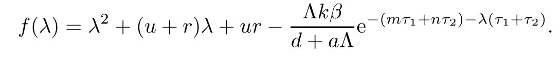
The basic reproductive number of viral infection for model(1.1)is

where R0denotes the average amount of the free virus released by the infected cells which are infected by the first virus.
It is easily proved that R0>1 implies>ur(d+aΛ)and k(β+bd)>
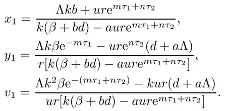
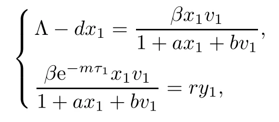
If R0>1,system(1.1)means that there is an immune-free equilibrium E1(x1,y1,v1,0,0),besides the equilibrium E0,where
Then,we obtain the antibody immune reproductive number R1and the CTL immune reproductive number R2for model(1.1)as follows:

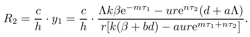
Here,R1denotes the average number of the antibody immune cells activated by the virus when virus infection is successful and CTL responses have not been established,and R2denotes the average number of the CTL immune cells activated by infected cells when virus infection is successful and antibody immune responses have not been established.
We know that R1>1 is equivalent to gv1?α>0,and R2>1 is equivalent to cy1?h>0.If R1>1,system(1.1)gives a unique infection equilibrium E2(x2,y2,v2,0,w2)with only antibody responses,where

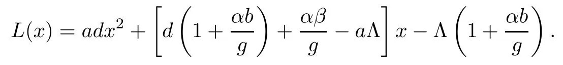
and x2is a unique positive zero point of the quadratic function
Next,we prove that each component of equilibrium E2is positive if R1>1.In fact,from
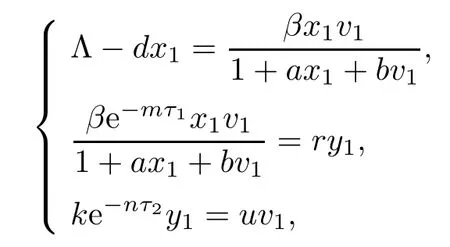
it is easy to show that

Therefore,if R1>1,we have

Thus,it follows that

From the expression of ω2,it follows that the existence of equilibrium E2is equivalent to
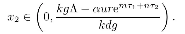
Noticing that L(0)<0,we know that the existence and uniqueness of equilibrium E2is equivalent to

Since
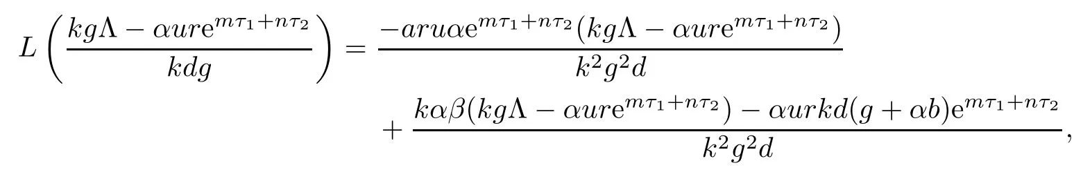
from R1>1,we have

Therefore,when R1>1,we obtain
If R2>1,with system(1.1)there exists a unique infection equilibrium E3(x3,y3,v3,z3,0)with only CTL responses,where

and x3is a unique positive root of the quadratic function

Next,we prove that each component of equilibrium E3is positive if R2>1.In fact,from
it is easy to show that

Therefore,if R2>1,we have

Thus,it follows that

From the expression of z3,it follows that the existence of equilibrium E3is equivalent to

Noticing that H(0)<0,we know that the existence and uniqueness of equilibrium E3is equivalent to
Since
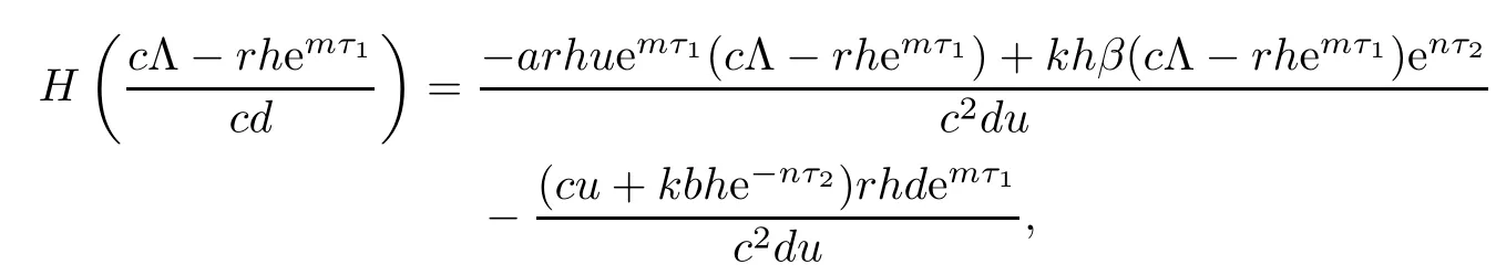
from R2>1,we have

Therefore,when R2>1,we obtain

Furthermore,we obtain the CTL immune competitive reproductive number R3and the antibody immune competitive reproductive number R4for model(1.1)as follows:
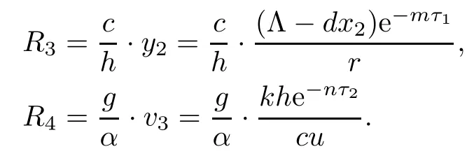
Here,R3denotes the average number of the CTL immune cells activated by infected cells under the condition that antibody immune responses have been established,and R4denotes the average number of the antibody immune cells activated by virus under the condition that CTL immune responses have been established.
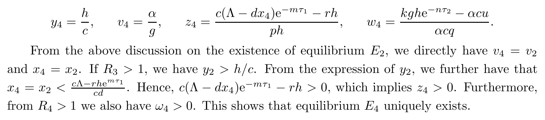
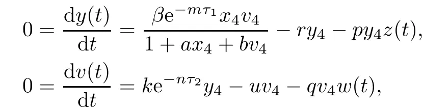
If R3>1 and R4>1,system(1.1)gives a unique infection equilibrium E4(x4,y4,v4,z4,w4)with CTL and antibody responses,where
3 Stability Analysis of Each Equilibrium
In this section,we discuss the global stability and instability for the infection-free equilibrium E0,immune-free equilibrium E1,and infection equilibrium E3with only CTL immune responses,and when τ3=0,the global stability for the infection equilibrium E2with only antibody responses and infection equilibrium E4with both CTL and antibody responses.
Let g(x)=x?1?lnx.Clearly,for x∈(0,+∞),g(x)is nonnegative and has the global minimum at x=1 and g(1)=0.
Theorem 3.1(i)If R0≤1,then the infection-free equilibrium E0(x0,0,0,0,0)is globally asymptotically stable;(ii)If R0>1,then E0(x0,0,0,0,0)is unstable.
Proof(i)Define a Lyapunov function
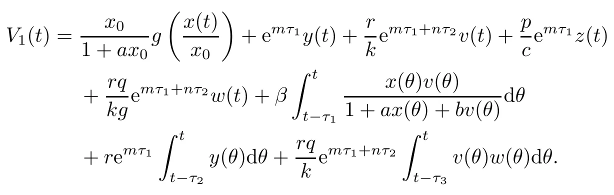
Clearly,V1(t)≥0,and V1(t)=0 if and only if x(t)=x0,y(t)=0,v(t)=0,z(t)=0 and ω(t)=0.
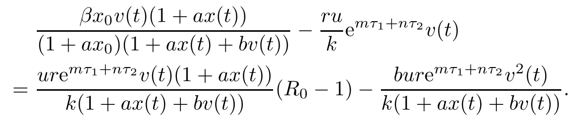
Then the time derivative of V1(t)along system(1.1)satisfies


Note that
(ii)The characteristic equation of the linearized system of model(1.1)at the equilibrium E0is

Clearly,equation(3.1)always has three negative real roots:λ1=?d,λ2=?α,λ3=?h.Hence,the stability of E0is determined by the roots of equation

Let
If R0>1,it is easy to show that
Hence,equation(3.2)has at least one positive real root in this case.Therefore,if R0>1,the equilibrium E0is unstable.This completes the proof. □
Theorem 3.2Let R0>1.
(i)If R1≤1 and R2≤1,then the immune-free equilibrium E1(x1,y1,v1,0,0)is globally asymptotically stable.
(ii)If R1>1 or R2>1,then E1(x1,y1,v1,0,0)is unstable.
Proof(i)Define a Lyapunov function

Clearly,V2(t)≥0,and V2(t)=0 if and only if x(t)=x1,y(t)=y1,v(t)=v1,z(t)=0 and w(t)=0.
Then the time derivative of V2(t)along system(1.1)satisfies
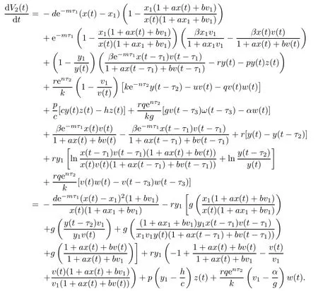
Note that


(ii)The characteristic equation of the linearized system of model(1.1)at the equilibrium E1is

where
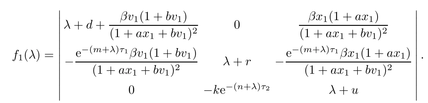
Let
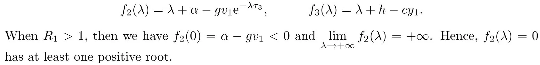
When R2>1,then we have h?cy1<0.Hence,f3(λ)=0 has one positive root λ?=cy1?h.
Therefore,when R1>1 or R2>1,E1is unstable.This completes the proof. □
Theorem 3.3Let R0>1 and R1>1.
(i)If R3≤1 and τ3=0,then the antibody response equilibrium E2(x2,y2,v2,0,w2)is globally asymptotically stable.
(ii)If R3>1,then E2(x2,y2,v2,0,w2)is unstable.
Proof(i)Define a Lyapunov function
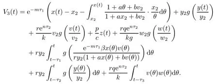
Clearly,V3(t)≥0,and V3(t)=0 if and only if x(t)=x2,y(t)=y2,v(t)=v2,z(t)=0 and ω(t)=ω2.
Then the time derivative of V3(t)along system(1.1)satisfies

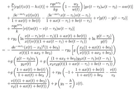
Note that
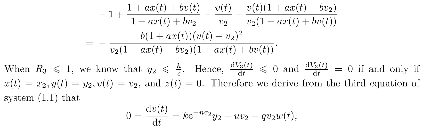
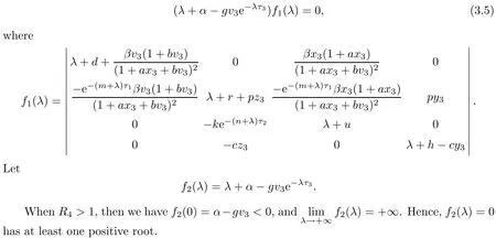
which yields w(t)=w2.From LaSalle’s invariance principle[31],we have that E2is globally asymptotically stable when R0>1,R1>1,R3≤1 and τ3=0.(ii)The characteristic equation of the linearized system of model(1.1)at the equilibrium E2is

where
Let
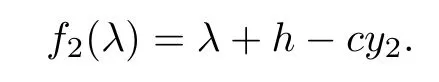
When R3>1,then we have f2(0)=h?cy2<0,and=+∞.Hence,f2(λ)=0 has at least one positive root.
Therefore,when R3>1,E2is unstable.This completes the proof. □
Theorem 3.4Let R0>1 and R2>1.
(i)If R4≤1,then the CTL immune response equilibrium E3(x3,y3,v3,z3,0)is globally asymptotically stable.
(ii)If R4>1,then E3(x3,y3,v3,z3,0)is unstable.
Proof(i)Define a Lyapunov function
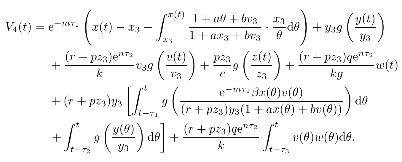
Clearly,V4(t)≥0,and V4(t)=0 if and only if x(t)=x3,y(t)=y3,v(t)=v3,z(t)=z3and ω(t)=0.
Then the time derivative of V4(t)along system(1.1)satisfies
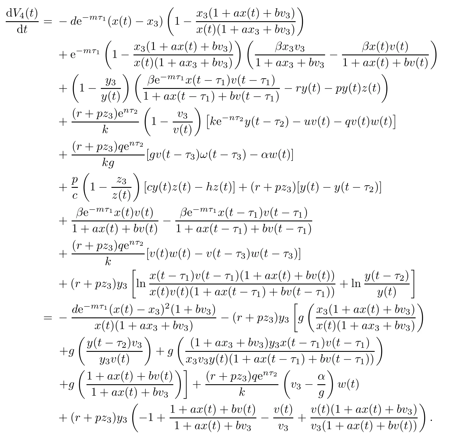
Note that

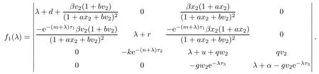
(ii)The characteristic equation of the linearized system of model(1.1)at the equilibrium E3is
Therefore,when R4>1,E3is unstable.This completes the proof. □
Theorem 3.5If R0>1,R2>1,R3>1,R4>1 and τ3=0,the interior equilibrium E4(x4,y4,v4,z4,w4)is globally asymptotically stable.
ProofDefine a Lyapunov function
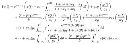
Clearly,V5(t)≥0,and V5(t)=0 if and only if x(t)=x4,y(t)=y4,v(t)=v4,z(t)=z4and ω(t)=ω4.
Then the time derivative of V5(t)along system(1.1)satisfies
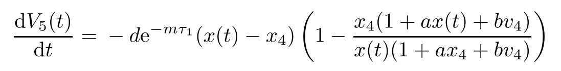
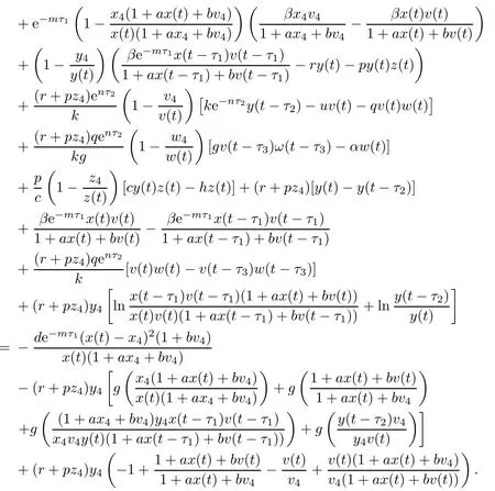
Note that
which yields z(t)=z4,w(t)=w4.From LaSalle’s invariance principle[31],we have that E4is globally asymptotically stable when R0>1,R2>1,R3>1,R4>1 and τ3=0.This completes the proof. □
4 Hopf Bifurcation Analysis of E2 and E4
4.1 Hopf bifurcation analysis of E2
By Theorem 3.3,we obtain the globally asymptotic stability of the equilibrium E2when τ1≥0,τ2≥0,τ3=0.However,when τ3>0,Hope bifurcation occurs at the equilibrium E2.When τ1>0,τ2>0,the calculation is too complicated.Hence,in order to simplify the calculation,we let τ1=0,τ2=0,τ3>0 in the discussions that follow.
From(3.4),the characteristic equation of the linearized system of model(1.1)at the equilibrium E2is

Letting λ=iω(ω>0)be a solution of equation(4.1),separating real and imaginary parts,it follows that

Squaring and adding the two equations of(4.2),we obtain that

where
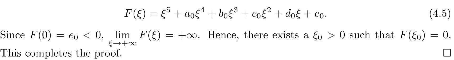
Letting ξ=ω2,equation(4.3)becomes

In what follows,some lemmas will be given to establish the existence of positive roots of equation(4.4).
Lemma 4.1If e0<0,then equation(4.4)has at least one positive root.
ProofDenote
Next,we will discuss the distribution of positive roots of equation(4.4)when e0≥0.The derivative of F(ξ)with respect to ξ is
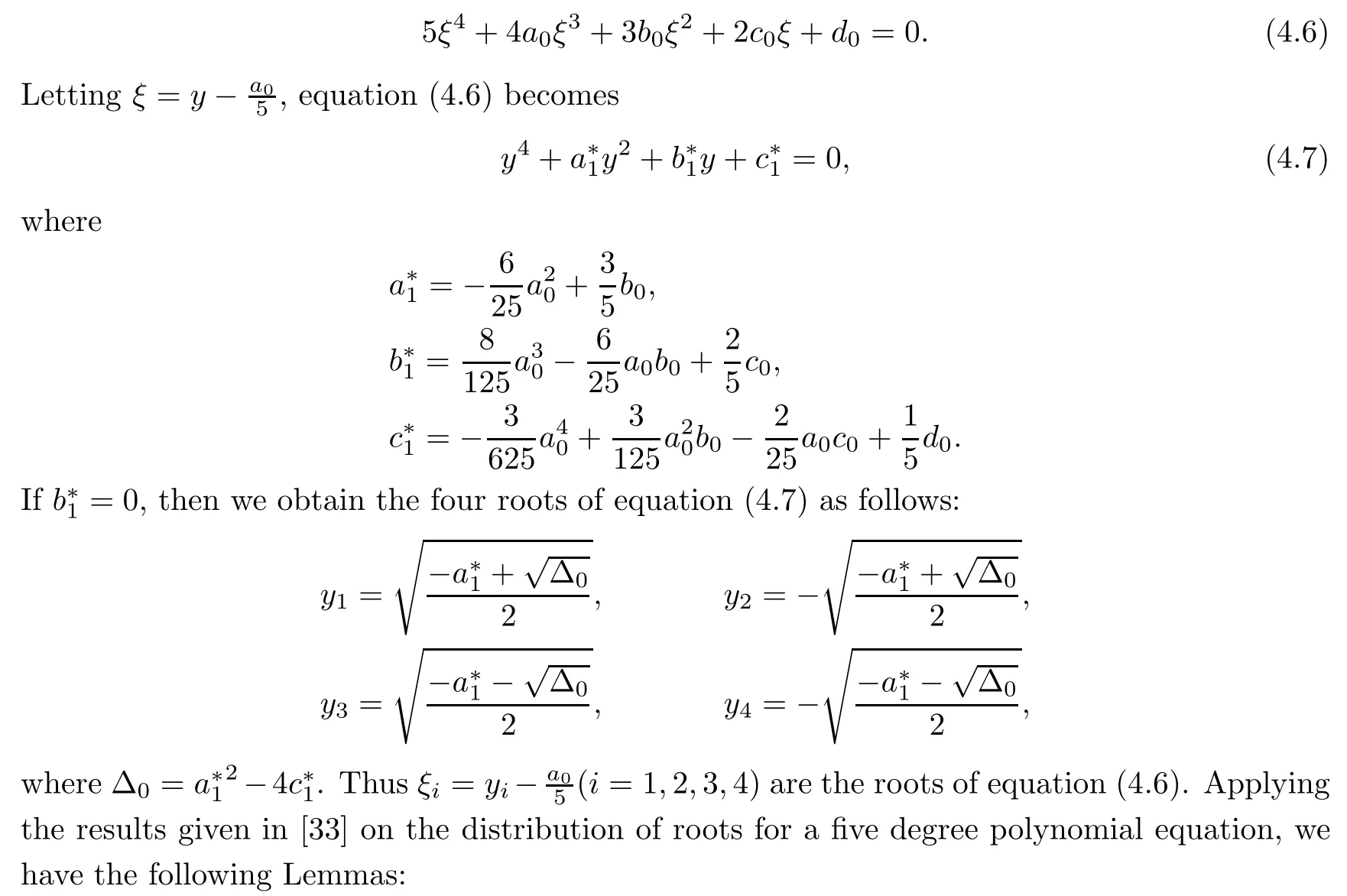
Lemma 4.2Suppose that e0≥0 and b?1=0.Then
(i)if Δ0<0,then equation(4.4)has no positive real roots;
(ii)if Δ0≥0,a?1≥0 and c?1>0,then equation(4.4)has no positive real roots;
(iii)if(i)and(ii)are not satisfied,then equation(4.4)has positive real roots if and only if there exists at least one ξ?∈{ξ1,ξ2,ξ3,ξ4}such that ξ?>0 and F(ξ?)≤0.
Denote
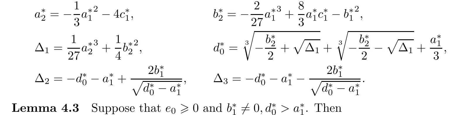
(i)if Δ2<0 and Δ3<0,then equation(4.4)has no positive real roots;
(ii)if(i)is not satisfied,then equation(4.4)has positive real roots if and only if there exists at least one ξ?∈{ξ1,ξ2,ξ3,ξ4}such that ξ?>0 and F(ξ?)≤0,where ξi=(i=1,2,3,4),and
Suppose that equation(4.4)has positive roots.Without loss of generality,we assume that it has m(1≤m≤5)positive roots,denoted by ξk,k=1,2,...,m.Then equation(4.3)has m positive roots ωk=k=1,2,...,m.
From equation(4.2),we have
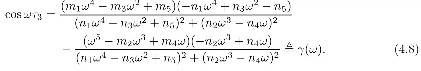
Thus,if we denote

From equation(4.3),we get

By equation(4.5),we have

Therefore,

This completes the proof. □
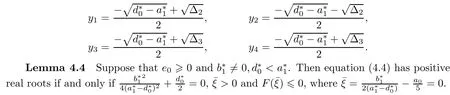
Summing up the above lemmas and the Hopf bifurcation theorem for functional differential equation[33],we get the following conclusion:
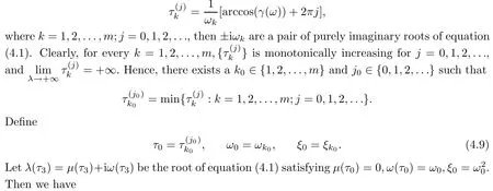
Theorem 4.6Let ξ0and ω0,τ0be defined by equation(4.9).

4.2 Hopf bifurcation analysis of E4
By Theorem 3.5,we obtain the globally asymptotic stability of the equilibrium E4when R0>1,R2>1,R3>1,R4>1 and τ3=0.From the theoretical analysis that follows,we will see that Hopf bifurcation occurs at the equilibrium E4when τ3>0.However,when τ1>0,τ2>0,the calculation is too complicated.Hence,in order to simplify the calculation,we also let τ1=0,τ2=0,τ3>0 in the ensuing discussions.
The characteristic equation of the linearized system of model(1.1)at the equilibrium E4is

Letting λ=iω(ω>0)be a solution of equation(4.10),separating real and imaginary parts,it follows that
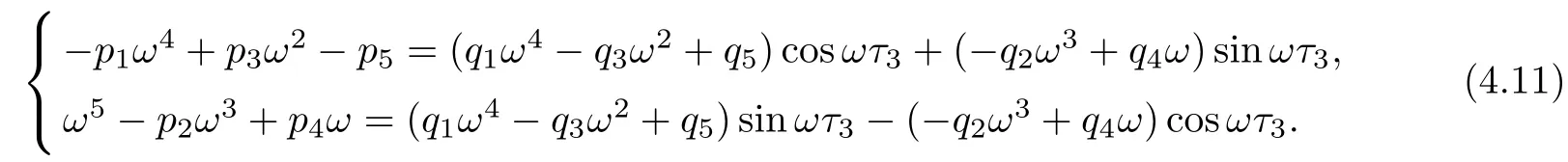
Squaring and adding the two equations of(4.11),we obtain that

where
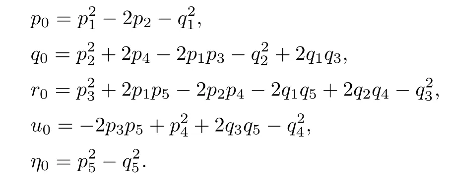
Letting ξ=ω2,equation(4.12)becomes

The derivative of H(ξ)with respect to ξ is

Denote
Applying the same method as Theorem 4.6,we have the following result:
Theorem 4.7Let ξ0and ω0,τ0be defined by equation(4.9).
5 Numerical Simulations
In Theorems 4.6 and 4.7,by using the theory of bifurcation,we have gather the existence of the Hopf bifurcation at equilibria E2and E4when τ1=0,τ2=0,τ3>0.However,when τ1>0,τ2>0,τ3>0,the theoretical analysis is very complicated.Thus,in what follows,by the numerical simulations it is shown that the Hopf bifurcation and stability switches occur at E2and E4as τ3increases.
Example 5.1In system(1.1),we choose a set of parameters as follows:
Λ=10,d=0.01,r=0.8,p=1,b=0.01,k=0.4,u=0.3,q=1,g=1.5,m=0.01,n=0.01,c=0.01,h=0.8,a=0.02,β=0.5,α=1,τ1=10,τ2=0.2.
By direct calculation,we obtain that E2(64.4132,10.5819,0.6667,0,6.0365),and R1=22.5403>1,R3=0.1323<1.From Figure 1 to Figure 4,with the increase of τ3,the dynamic behavior of the equilibrium E2will change;that is,Hopf bifurcation appears.
Figure 1 When τ3=0.1,infection equilibrium E2 with only the antibody response of system(1.1)is locally asymptotically stable

Figure 2 When τ3=1.5,infection equilibrium E2 with only the antibody response of system(1.1)is unstable
Figure 3 When τ3=8.95,infection equilibrium E2 with only the antibody response of system(1.1)is locally asymptotically stable
Example 5.2In system(1.1),we choose a set of parameters as follows:
Λ=10,d=0.01,r=0.5,p=1,b=0.01,k=0.4,u=0.3,q=1,g=1.5,m=0.01,n=0.01,c=0.1,h=0.15,a=0.02,β=0.5,α=1,τ1=1,τ2=4.
By direct calculation,we obtain that E4(64.4132,1.5,0.6667,5.6752,0.5647),and R1=37.2577>1,R3=12.2275>1,R4=2.8537>1.From Figure 5 to Figure 8,with the increase of τ3,the dynamic behavior of the equilibrium E4will change as follows:locally asymptotically stable→unstable→locally asymptotically stable→unstable;that is,Hopf bifurcation appears.
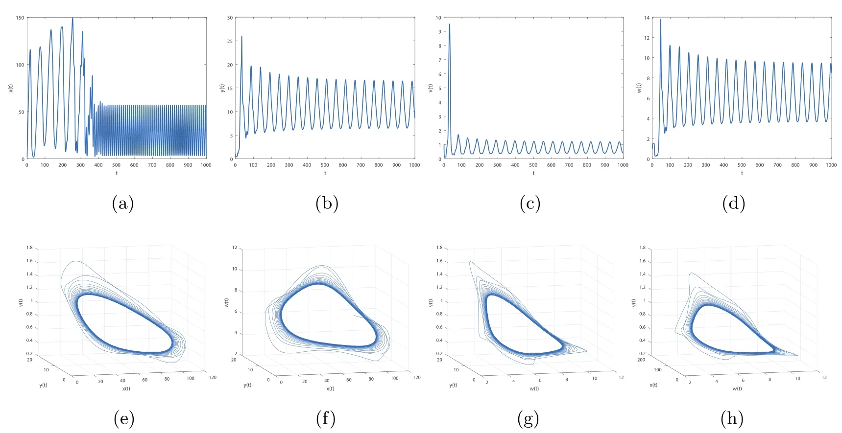
Figure 4 When τ3=10,infection equilibrium E2 with only the antibody response of system(1.1)is unstable
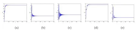
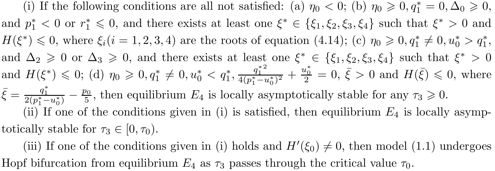
Figure 5 When τ3=0.001,the infection equilibrium E4,with both the antibody and CTL responses of system(1.1),is locally asymptotically stable
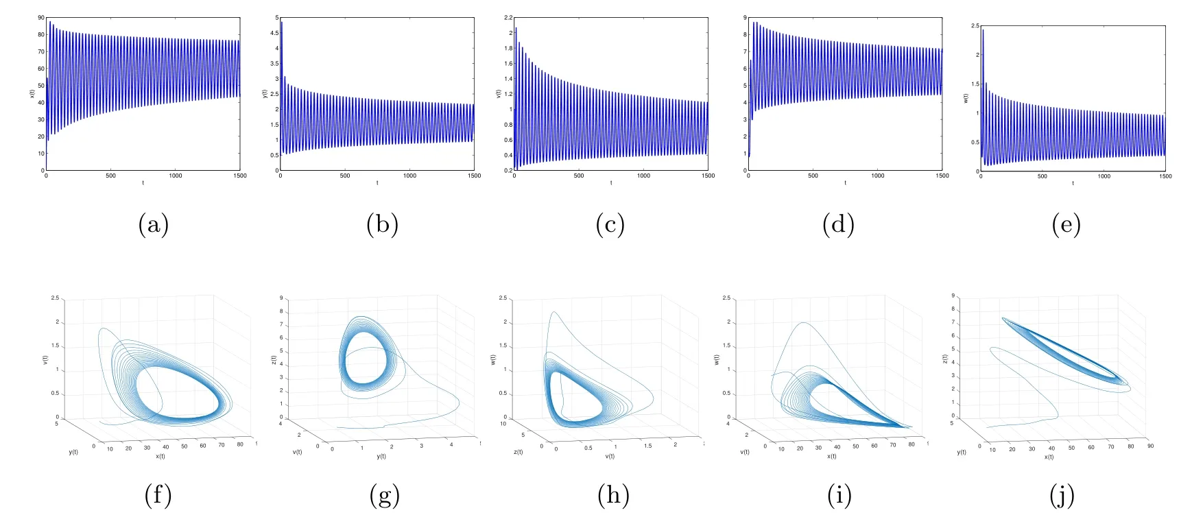
Figure 6 When τ3=2,the infection equilibrium E4,with both the antibody and CTL responses of system(1.1),is unstable

Figure 7 When τ3=22.7,the infection equilibrium E4,with both the antibody and CTL responses of system(1.1),is locally asymptotically stable
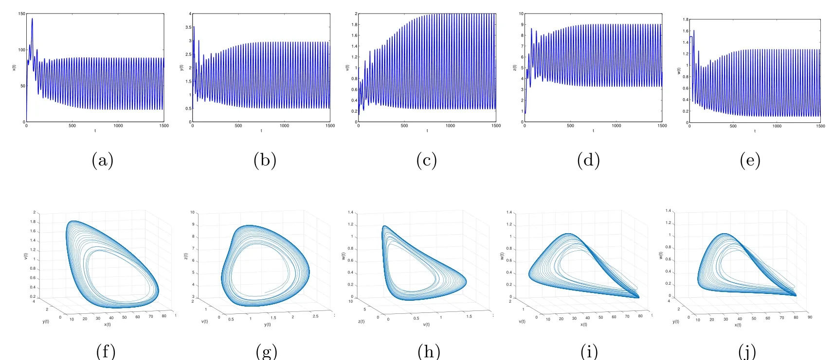
Figure 8 When τ3=30,the infection equilibrium E4,with both the antibody and CTL responses of system(1.1),is unstable
6 Discussion
In this paper,a delayed viral infection model with CTL immune response and antibody immune response have been considered,along with three delays:the intracellular delay,virus replication delay and the antibody delay.We assumed that the production of CTL immune response depends on the infected cells and CTL cells,and the production of antibody response depends on the virus and antibody cells.
In Section 2,we presented that the solutions of model(1.1)are bounded,and showed that this model exists with five possible equilibria:an infection-free equilibrium E0,an immune-free equilibrium E1,an infection equilibrium E2with only antibody response,an infection equilibrium E3with only CTL response,and an infection equilibrium E4with both CTL and antibody responses,depending on the threshold values.In this paper,we have presented five threshold values:the basic reproductive rate of viral infection R0,the antibody immune reproductive rate R1,the CTL immune reproductive rate R2,the CTL immune competitive reproductive rate R3,and the antibody immune competitive reproductive rate R4.These determine not only the existence of the equilibrium point,but also the dynamic behavior of the model.
In Section 3,the results have shown that when R0≤1,E0is globally asymptotically stable for any time delay τ1,τ2,τ3≥0,which means that the viruses are cleared,and CTL immunity and antibody immunity are not active.Moreover,we found that R0can be reduced by increasing the delay τ1and τ2;that is,we can reduce the average amount of viral infection.When R0>1,R1≤1 and R2≤1,E1is globally asymptotically stable for any time delay τ1,τ2,τ3≥0,which means that the infection becomes chronic but with no persistent CTL immune responses and antibody responses.When R0>1,R2>1,and R4≤1,E3is globally asymptotically stable for any time delay τ1,τ2,τ3≥0,which means that the infection becomes chronic with persistent CTL immune responses,but the virus loads cannot activate the antibody responses.The above results show that delays τ1,τ2,and τ3do not impact the global asymptotic properties of E0,E1,E3,and therefore the possibility of Hopf bifurcation is ruled out.With respect to the analysis of E2,E4,we considered special cases τ1≥0,τ2≥0,and τ3=0.When R0>1,R1>1,and R3≤1,E2is globally asymptotically stable,which means that the infection becomes chronic with persistent antibody responses,but the infected cells cannot stimulate and activate CTL immune responses.When R0>1,R2>1,R3>1,and R4>1,E4is globally asymptotically stable,that is,uninfected target cells,infected cells,free virus,CTL response cells and antibody response cells coexist in vivo.From the above results,we see that delays τ1,τ2do not impact upon the global asymptotic properties of E2,E4,but the antibody delay τ3can impact upon the stability of E2,E4.
In Section 4,by using the bifurcation theory,a detailed analysis on the local asymptotic stability and the existence of Hopf bifurcation at the equilibrium point E2and E4was carried out when τ3>0.When τ1>0,τ2>0,the calculation proved to be too complicated.Hence,in order to simplify the calculation,we let τ1=0,τ2=0,τ3>0.In Section 5,by means of numerical simulations,it was shown that Hopf bifurcation occurs at the equilibrium points E2and E4as the antibody delay τ3increases.From Figures 1 to 8,as τ3increases,we saw that the dynamic behavior of E2and E4will change as follows:locally asymptotically stable→unstable→locally asymptotically stable→unstable;that is,Hopf bifurcation appears.
Summarizing these results,we point out that the intracellular delay τ1and virus replication delay τ2do not impact the stability of all the equilibria,but the antibody delay τ3markedly affects the stability of the antibody response equilibrium E2and the interior equilibrium E4.This indicates that the antibody delay τ3plays a negative part in the diseases prevalence and control.In this paper,we have extended the conclusions of the model in[30]with a saturation incidence rate to a Beddington-DeAngelis infection rate,and have successfully completed the questions raised by Miao[29].We also point out the essential difference between our results and the results in[29],by which our work was motivated.In[29],CTL immune delay was considered,and the conclusion was that immune response delay markedly affects the stability of CTL response equilibrium and the interior equilibrium.In our model,however,the antibody delay was discussed,which is precisely the question raised in[29],but not studied,and a different conclusion has been drawn:the antibody delay markedly affects the stability of the antibody response equilibrium and the interior equilibrium.
猜你喜歡
Chinese Physics B(2023年12期)2023-12-15 11:47:54
Chinese Physics B(2023年11期)2023-12-02 09:29:14
Chinese Physics B(2023年11期)2023-12-02 09:22:36
今日農(nóng)業(yè)(2022年15期)2022-09-20 06:55:04
Chinese Physics B(2021年1期)2021-01-21 02:07:10
詩(shī)潮(2019年11期)2019-11-23 12:20:12
知音海外版(下半月)(2019年3期)2019-06-11 12:09:56
知音海外版(上半月)(2019年3期)2019-03-29 06:11:32
大眾文藝(2019年3期)2019-01-24 13:39:44
學(xué)校教育研究(2018年1期)2018-10-21 02:10:47
 Acta Mathematica Scientia(English Series)2021年3期
- Acta Mathematica Scientia(English Series)的其它文章
- ANALYSIS OF THE GENOMIC DISTANCE BETWEEN BAT CORONAVIRUS RATG13 AND SARS-COV-2 REVEALS MULTIPLE ORIGINS OF COVID-19?
- BILINEAR SPECTRAL MULTIPLIERS ON HEISENBERG GROUPS?
- ON SCHWARZ-PICK TYPE INEQUALITY FOR MAPPINGS SATISFYING POISSON DIFFERENTIAL INEQUALITY?
- EXISTENCE AND UNIQUENESS OF THE GLOBAL L1 SOLUTION OF THE EULER EQUATIONS FOR CHAPLYGIN GAS?
- UNIQUENESS OF THE INVERSE TRANSMISSION SCATTERING WITH A CONDUCTIVE BOUNDARY CONDITION?
- THE FIELD ALGEBRA IN HOPF SPIN MODELS DETERMINED BY A HOPF ?-SUBALGEBRA AND ITS SYMMETRIC STRUCTURE?