
DYNAMICS FOR AN SIR EPIDEMIC MODEL WITH NONLOCAL DIFFUSION AND FREE BOUNDARIES?
2021-09-06 07:54:16趙孟
關(guān)鍵詞:趙孟
(趙孟)
College of Mathematics and Statistics,Northwest Normal University,Lanzhou 730070,China School of Mathematics and Statistics,Lanzhou University,Lanzhou 730000,China E-mail:zhaom@nwnu.edu.cn
Wantong LI (李萬(wàn)同)?
School of Mathematics and Statistics,Lanzhou University,Lanzhou 730000,China E-mail:wtli@lzu.edu.cn
Jiafeng CAO (曹佳峰)
Department of Applied Mathematics,Lanzhou University of Technology,Lanzhou 730050,China E-mail:caojf07@lzu.edu.cn
Abstract This paper is concerned with the spatial propagation of an SIR epidemic model with nonlocal diffusion and free boundaries describing the evolution of a disease.This model can be viewed as a nonlocal version of the free boundary problem studied by Kim et al.(An SIR epidemic model with free boundary.Nonlinear Anal RWA,2013,14:1992–2001).We first prove that this problem has a unique solution de fined for all time,and then we give sufficient conditions for the disease vanishing and spreading.Our result shows that the disease will not spread if the basic reproduction number R0<1,or the initial infected area h0,expanding abilityμ,and the initial datum S0are all small enough when.Furthermore,we show that if,the disease will spread when h0is large enough or h0is small butμis large enough.It is expected that the disease will always spread when R0,which is different from the local model.
Key words SIR model;nonlocal diffusion;free boundary;spreading and vanishing
1 Introduction
In mathematical epidemiology,one of the most important models is the classical SIR model,which receives great attention.In this model,according to the stage of infection,the population is separated into three classes:susceptible,infectious and recovered individuals,denoted byS,I
andR
,respectively.Assuming that the disease incubation period is negligible so that each susceptible individual becomes infectious and later recovers having acquired a permanent or temporary immunity,then the classical SIR model can be governed by


R
<
1,and remain endemic ifR
>
1.Obviously,(1.1)ignores the spatial diffusion of the population.Motivated by this factor,Kuniya and Wang[21]studied the corresponding spatial diffusion problem,and obtained a result similar to[15]for some special cases.To describe how an epidemic spreads in space,spreading speed is an useful approach.We refer to Hosono and Ilyas[16]for the spreading speed of a corresponding spatial diffusion problem.However,the works of Kuniya and Wang[21]and Hosono and Ilyas[16]cannot describe precisely the spreading front of the disease.This shortcoming can be overcome by considering the problem over a moving domain,resulting in the free boundary problem.Kim et al.[20]introduced the free boundary in order to consider the corresponding spatial diffusion problem;that is to say,they assume that the populationsS,I
andR
disperse randomly,and the range of infected area is assumed to be a moving interval,B
(0).This model has the form
where the free boundaries satisfy the famous Stefan condition.Kim et al.first proved the existence and uniqueness of the global solution,and then gave the sufficient conditions for the disease vanishing or spreading:
(i)IfR
<
1,thenh
<
∞.(ii)IfR
>
1,then there existh
andh
such that(a)ifh
>h
,thenh
=∞;(b)ifh
≤h
,then there existsμ
>
0 such thath
<
∞for 0<μ<μ
,whereR
is given by(1.2).Moreover,ifh
<
∞,then
S,I
andR
if vanishing happens.For(1.3),the deduction of free boundary conditionh
(t
)=?μI
(t,h
(t
))can be found in[2].Du and Lin[6]were the first to use this condition to consider a logistic type of local diffusion model with a free boundary.After this work,many local diffusion problems with a free boundary were investigated;see[7,8,10–14,18,19,22,26–29,32–35]and the references therein.Recently,Cao et al.[3]proposed a nonlocal version of[6],and successfully extended many basic results of[6]to the nonlocal model.For the spreading-vanishing criteria,the results in[3]revealed signi ficant differences from the local diffusion model in[6].Very recently,Du et al.[5]investigated the spreading speed of the nonlocal model in[3]and proved that the spreading may or may not have a finite speed,depending on whether a certain condition is satis fied by the kernel functionJ
.From these results,we can see that there are striking differences between the local and nonlocal diffusion models.Motivated by the work[3],many researchers investigated other problems with nonlocal diffusion and free boundaries;for example,Du et al.[9]considered a class of two species of Lotka-Volterra models with nonlocal diffusion and common free boundaries,Li et al.[24]discussed a class of free boundary problem in relation to ecological models with nonlocal and local diffusions,Zhao et al.[36]studied a degenerate epidemic model with nonlocal diffusion and free boundaries,Cao et al.[4]considered the dynamics of a Lotka-Volterra competition model with nonlocal diffusion and free boundaries,Wang and Wang[30,31]studied free boundary problems with nonlocal and local diffusions,and[23]considered the dynamics of nonlocal diffusion systems with different free boundaries,and so on.
Inspired by the above works about nonlocal diffusion,the main purpose of this paper is to extend the results in[20]into the free boundary problem with nonlocal diffusion.For simplicity,we assume that the spatial region is one dimensional.If the spatial movement is described by a nonlocal diffusion operator(see[1,25])andS,I
andR
have the same diffusion rate,then we can propose the nonlocal variation of(1.3)as follows:
d,μ
andh
are positive constants.It is assumed that the kernel functionJ
:R→R is continuous and nonnegative,and has the properties
S
(x
)belongs to
I
(x
)andR
(x
)belong to
h
,h
]represents the initial infected area.We note that the detailed derivation of the free boundary conditionsh
(t
)andg
(t
)in(1.4)can be found in[3].We will show that(1.4)has a unique solution de fined for all time,and then determine its longtime dynamical behaviour.It is emphasized that we apply the approach in[3,9,36]to deal with(1.4),which is different from[20].Note that the equations forS
andI
are fully decoupled fromR
in(1.4).Although we only need to consider the sub-system forS
andI
,the reaction functions are different from the above mentioned works considering systems with nonlocal diffusion.As a result,the arguments in this paper will be a little different.The main results of this paper are the following theorems:Theorem 1.1
Suppose that(J)holds.Then,for any givenh
>
0,S
∈XandI
,R
∈X,problem(1.4)has a unique positive solution(S
(t,x
),I
(t,x
),R
(t,x
),g
(t
),h
(t
))de fined for allt>
0.It is easily seen thath
(t
)is monotonically increasing and thatg
(t
)is monotonically decreasing.Therefore
R
is given by(1.2),so we haveTheorem 1.2
Let the conditions of Theorem 1.1 hold and let(S,I,R,g,h
)be the solution of(1.4).Assume further thatJ
(x
)>
0 in R.Then we have
l
is determined by an eigenvalue problem(see(3.6)).Finally,we first explain the differences between the model with nonlocal diffusion and the one with local diffusion based on the work[3,5,6].
Remark 1.3
We note that local diffusion is only suitable to describe short-range in the dispersal,however,nonlocal diffusion can be used to study long-range factors in the dispersal by choosing the kernel functionJ
properly.Mathematically,the results in[3]showed that if the diffusion rate of the species is small enough,then spreading will always happen,which is very different from that which is described in[6].On the other hand,the results in[5]showed that the spreading may have an in finite speed,which is another difference from the local model.Biologically,this means that nonlocal diffusion of the species increases the chance of species spreading,compared with the case that the species only diffuses randomly.For our results,we have the following two remarks discussing the differences between the local and nonlocal model:

Remark 1.5
Depending on the choice of the kernel function in the nonlocal diffusion operator,Du et al.[5]showed that the spreading speed of the nonlocal model in[3]is accelerated.It is expected that a similar result holds for(1.4),which presents an interesting problem.To check this result,we should first obtain the longtime behavior of(1.4)for when spreading happens.We will consider this in the future.The rest of this paper is organised as follows:in Section 2 we prove Theorem 1.1,namely,problem(1.4)has a unique solution de fined for allt>
0;the longtime dynamical behaviour of(1.4)is investigated in Section 3,where Theorem 1.2 is proved.2 Global Existence and Uniqueness
Throughout this section,we assume thath
>
0,S
∈XandI
,R
∈X.For any givenT>
0,we first introduce the following notations: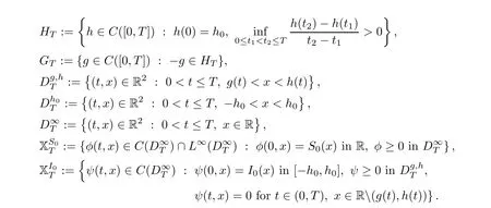
Just as in[3],we first prove the following lemma:
Lemma 2.1
For any givenT>
0 and(g,h
)∈G
×H
,the problem
μ
=min{μ
,μ
,μ
}.Proof
If we can obtain the existence and uniqueness of(S,I
),then the existence and uniqueness ofR
can follow from[36,Lemma 2.2].Hence we only need to consider problem
S,I
).Letf
(S,I
)=b
?βSI
?μ
S
andf
(S,I
)=βSI
?αI
?μ
I
.Sincef
(0,I
)/=0,andS
is de fined in(0,T
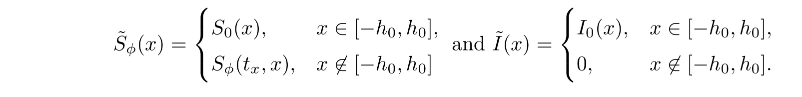
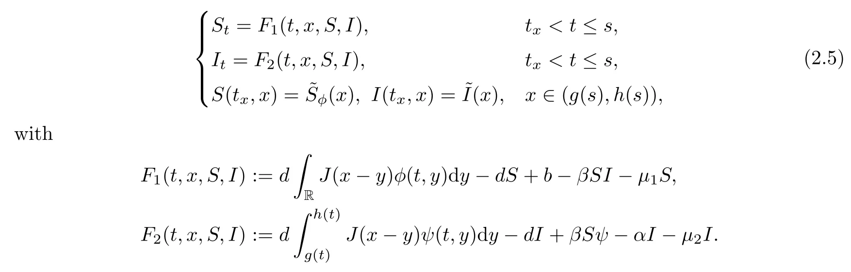
]×R,the corresponding result in[9]does not cover this case.However,we can deal with this by making some considerable changes.Here we give the details.Step 1
The parameterised ODE problems.For any givenx
∈R ands
∈(0,T
],de fine
I
(t,x
)=0.Consider the following ODE initial value problem: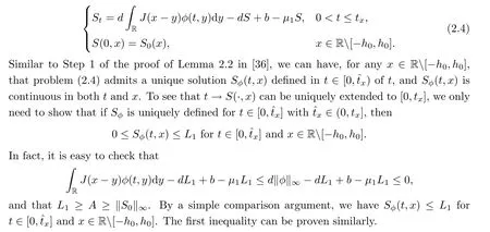
x
∈(g
(s
),h
(s
))andt
∈[t
,s
].De fine
Consider the ODE problem
S
,I
)∈[0,L
]×[0,L
],
F
(t,x,S,I
)is Lipschitz continuous in(S,I
)for(S
,I
)∈[0,L
]×[0,L
],and is uniformly continuous forx
∈(g
(s
),h
(s
))andt
∈[t
,s
].Additionally,F
(t,x,S,I
)is continuous in all its variables in this range.By the fundamental theorem of ODEs,problem(2.5)admits a unique solution(S
(t,x
),I
(t,x
))de fined in some interval[t
,s
)oft
,and(S
(t,x
),I
(t,x
))is continuous in botht
andx
.To claim thatt
→(S
(t,x
),I
(t,x
))can be uniquely extended to[t
,s
],we should show that if(S
,I
)is uniquely de fined fort
∈[t
,t
?]with?t
∈(t
,s
],then
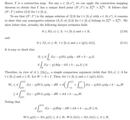
It is easy to check that

L
≥‖S
‖andL
≥‖I
‖,it follows from a simple comparison argument thatS
(t,x
)≤L
,I
(t,x
)≤L
int
∈[t
,t
?].The left part can be obtained similarly by usingF
(t,x,
0,
0)≥0.Step 2
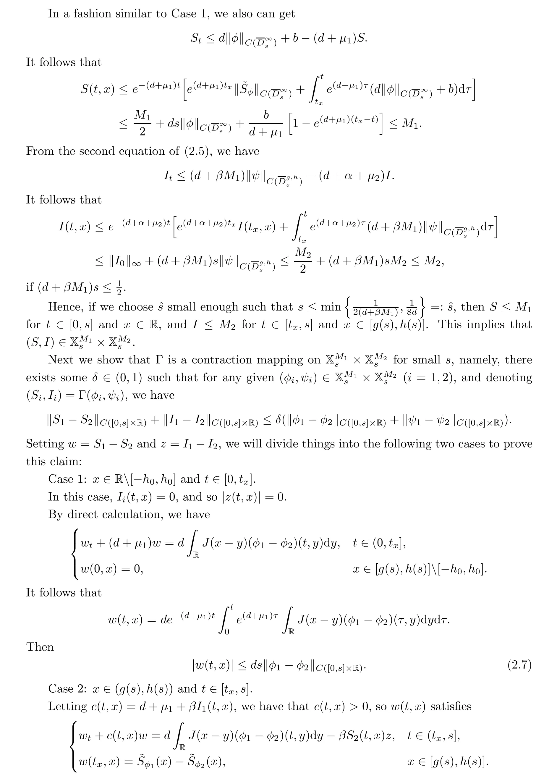
A fixed point theorem.For anys
∈(0,T
),we denote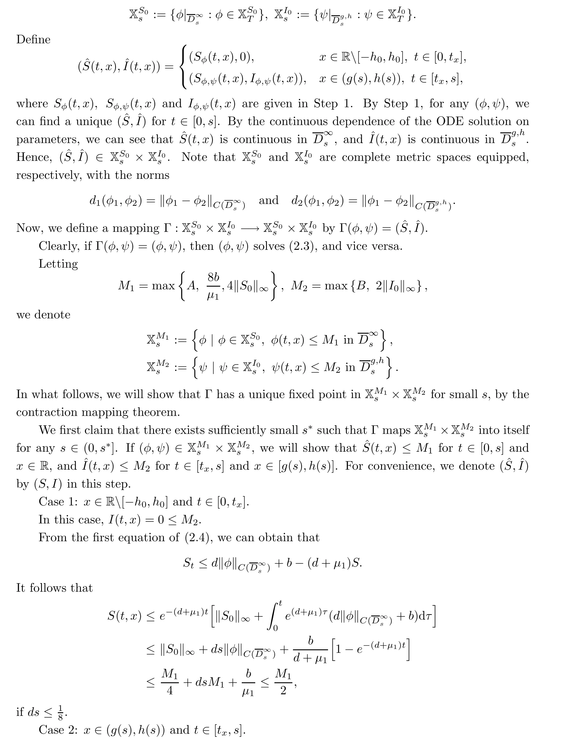

S
‖+‖I
‖≤B
,we can apply a simple comparison argument to see thatW
(t,x
)≤B
fort
∈[0,s
]andx
∈[g
(t
),h
(t
)].Hence,(2.11)holds.We have thus proved that for anys
∈(0,s
],(2.3)has a unique solution fort
∈[0,s
].Step 3
Extension of the solution.
Proof of Theorem 1.1
Following the approach of[3],we will make use of Lemma 2.1 and a fixed point argument to finish this proof.For any givenT>
0 and(g
,h
)∈G
×H
,it follows from Lemma 2.1 that(2.1)with(g,h
)=(g
,h
)has a unique solution(S
,I
,R
).Using suchI
(t,x
),we can de fine(g
?,
?h
)fort
∈[0,T
]by
J
(0)>
0,there exist constants?
∈(0,h
/
4)andδ
such that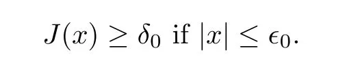
T
=T
(μ,B,h
,?
,I
,J
)>
0 and anyT
∈(0,T
],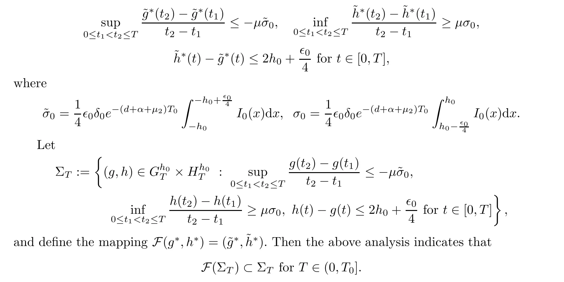
T
∈(0,T
],F has a unique fixed point(g
,h
)in Σ,so(S
,I
,R
,g
,h
)clearly is a solution of(1.4)fort
∈[0,T
].We will then show that this is the unique solution of(1.4)and that it can be extended uniquely to allt>
0.We will complete this task in several steps.Step 1
We show that,for sufficiently smallT
∈(0,T
],F has,by the contraction mapping theorem,a unique fixed point in Σ.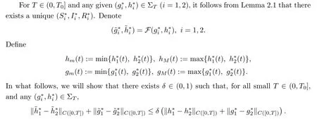
C
depending on(μ,h
,B
)such that
t
∈(0,T
],
C
depending on(d,α,β,μ
,A,B
).By[36,(2.16)],we have
T
≤1.Then the inequalities(2.15),(2.16)and(2.17)yield,for the casex
∈[?h
,h
(t
)],that
C
does not depend onT
and(t
,x
).Whenx
∈[g
(t
),
?h
),we can show that this inequality still holds.SinceZ
(t
,x
)=0 fort
∈[0,T
]andx
∈R[g
(t
),h
(t
)],we have
T
∈(0,T
?],F is a contraction mapping on Σ.Hence,F has a unique fixed point(g,h
)in Σ,which gives a nonnegative solution(S,I,R,g,h
)of(1.4)fort
∈(0,T
].Step 2
To show that(S,I,R,g,h
)is the unique solution of(1.4)fort
∈(0,T
],we should show that(g,h
)∈Σhold for any solution(S,I,R,g,h
)of(1.4)de fined int
∈(0,T
].This can be shown by the same argument as in Step 3 of the proof in[3,Theorem 2.1].Let(S,I,R,g,h
)be an arbitrary solution of(1.4)de fined fort
∈(0,T
].Then

Step 3
Extension of the solution of(1.4)tot
∈(0,
∞).
Firstly,we can show,as above,that


3 Spreading and Vanishing


Proof
Applying Lemma 3.1,we can prove this lemma by the same argument as in[3,Theorem 3.1]and[36,Lemma 3.2].Here we omit the proof.
Lemma 3.3
Ifθ<
0,or equivalently,R
<
1,thenh
?g
<
∞,and
Proof
We first prove(3.1).We note thatS
(t,x
)satis fies


h
?g
<
∞by lettingt
→∞.For the caseθ>
0,or equivalently,R
>
1,we de fine the operator L+θ
by
θ
is given by
Lemma 3.4
Assume thatJ
(x
)satis fies(J),and thatJ
(x
)>
0 in R.Let(S,I,R,g,h
)be the solution of(1.4).If 0<θ<d
andh
?g
<
∞,then
Proof
By the same arguments as in[9],we can have that


δ
small enough such thatδφ
(x
)≤I
(T
,x
)forx
∈[g
+?,h
??
],then we can use[3,Lemma 3.3]and a simple comparison argument to obtain
This is in contradiction to(3.2).Thus we have proven(3.3).
We next consider the case 0<θ<d.
In this case,it follows from[3,Proposition 3.4]that there existsl
such that

Proof
(i)Arguing indirectly,we assume thath
?g
>l
.Since 0<θ<d
,we haveλ
(L+θ
)>
0.This is in contradiction to(3.3).(ii)This conclusion follows directly from(i).
(iii)By using[9,Lemma 3.9],we can have that there existsμ
such thath
?g
=∞forμ>μ
.Now we prove the remaining part.Since 2h
<l
,we haveλ
(L+θ
)<
0.There exists some smallε
such thath
:=h
(1+ε
)satis fies

K
large enough such that
δ
determined above,we chooseK
such that
猜你喜歡
中國(guó)書(shū)法(2023年6期)2023-07-25 13:25:21
書(shū)畫(huà)世界(2022年4期)2022-06-13 08:25:13
書(shū)畫(huà)世界(2021年6期)2021-08-23 07:20:35
美與時(shí)代·下(2021年2期)2021-05-17 17:32:25
書(shū)畫(huà)世界(2021年3期)2021-04-28 17:00:50
書(shū)畫(huà)世界(2021年3期)2021-04-28 04:16:28
藝苑(2019年3期)2019-07-11 04:49:34
少兒美術(shù)·書(shū)法版(2017年9期)2017-06-28 08:20:56
老年教育(2017年4期)2017-05-10 05:27:34
絲路藝術(shù)(2017年6期)2017-04-18 13:59:16
 Acta Mathematica Scientia(English Series)2021年4期
- Acta Mathematica Scientia(English Series)的其它文章
- REGULARITY OF WEAK SOLUTIONS TO A CLASS OF NONLINEAR PROBLEM?
- EXISTENCE TO FRACTIONAL CRITICAL EQUATION WITH HARDY-LITTLEWOOD-SOBOLEV NONLINEARITIES?
- A DIFFUSIVE SVEIR EPIDEMIC MODEL WITH TIME DELAY AND GENERAL INCIDENCE?
- ON A COUPLED INTEGRO-DIFFERENTIAL SYSTEM INVOLVING MIXED FRACTIONAL DERIVATIVES AND INTEGRALS OF DIFFERENT ORDERS?
- CLASSIFICATION OF SOLUTIONS TO HIGHER FRACTIONAL ORDER SYSTEMS?
- ENERGY CONSERVATION FOR SOLUTIONS OF INCOMPRESSIBLE VISCOELASTIC FLUIDS?