Empirical Likelihood for Partially Linear Models Under Associated Errors

LI Yinghua(李英華), QIN Yongsong(秦永松)

( School of Mathematics and Statistics, Guangxi Normal University, Guilin 541004, China)

Abstract: In this paper, we use blockwise empirical likelihood (EL) technique to construct confidence regions for the regression coefficients in a partially linear models under stationary and associated errors.It is shown that the blockwise EL ratio statistic is asymptotically χ2-type distributed, which is used to construct EL-based confidence regions for the regression coefficients.Further, the results from a simulation study on the finite sample are also presented.

Key words: Partially linear model; Blockwise empirical likelihood; Associated sample;Confidence region

1.Introduction

Random variables{ηi,1 ≤i ≤n}are said to be positively associated(PA),or associated,if for any real-valued coordinatewise nondecreasing functions f and g, Cov(f(η1,η2,··· ,ηn),g(η1,η2,··· ,ηn)) ≥0, whenever this covariance exists.Infinitely many r.v.s.are said to be associated, if any finite subset of them is a set of associated.

The partially linear model was introduced by Engle et al.[6]to study the effect of weather on electricity demand, which is a natural compromise between the linear model and the fully nonparametric model.It allows only some of the predictors to be modeled linearly,with others being modeled nonparametrically.Due to its broad applications, the partially linear model has been studied extensively under independent observations.WANG and JING[7], QIN[8]and SHI and LAU[9]have given the construction of the empirical likelihood (EL) confidence region on β in the case of independent observations.

Consider the following partially linear model

where yi’s are scalar response variables, xi∈Rrand ti∈[0,1] are fixed design points, β ∈Rris a vector of unknown parameter, g(·) is the unknown regression function defined on [0,1]and errors ?i∈R are the random variables.In this paper, we assume that ?1,··· ,?nare stationary associated random errors with E?1=0,0<<∞.We will construct the EL confidence regions for β using the blocking technique in the following.

Here we mention some literatures related to the EL method.Kitamura[10]first proposed blockwise EL method to construct confidence intervals for parameters with mixing samples.Nordman et al.[11]proposed to use blockwise EL method to construct confidence intervals for the mean of a long-range dependent process.CHEN and WONG[12]developed a blockwise EL method to construct confidence intervals for quantiles with mixing samples.QIN and LI[13]used the blockwise EL method to construct confidence regions for the regression parameters in a linear model under negatively associated errors.Recently, QIN[14]and JIN and LEE[15]developed the EL method for spatial cross-sectional data models.LI et al.[16]extended the EL method proposed by QIN[14]and JIN and LEE[15]to spatial panel data models.For the partially linear models, LIN and WANG[17]used the blockwise EL for partially linear models under negatively associated(NA)errors and showed that the EL ratio statistic for the regression coefficients is asymptotically χ2distributed.

Negative association of random variables occurs in a number of important cases, but it has not been as popular as positive association.[2]On the other hand, it is much more difficult technologically to deal with PA samples than NA samples as there exist nice moment inequalities for sums of NA sequences and there are no nice moment inequalities for sums of PA sequences.It is therefore worth studying the construction of the EL-based confidence regions for the regression parameters in a partially linear model under associated errors.

The rest of this paper is organized as follows.The main results of this paper are presented in Section 2.Results of a simulation study on the finite sample performance of the proposed confidence intervals are reported in Section 3.Some lemmas to prove the main results and the proofs of the main results are presented in Section 4.

2.Main Result

Similar to [19], one can obtain the (?2log) blockwise EL ratio statistic

where λ(β)∈Rris determined by

Remak 1The usual weight function is Pristley and Chao weight[20]with Wni(u) ={(ti?ti?1)/h}Kh(u ?ti), where K(·) is a kernel function, h = hnis the bandwidth and Kh(t) = K(t/h).By appropriately selecting K, h and the design points {ti,xi,1 ≤i ≤n},Assumptions A3 and A4 can be satisfied.

We now state the main result in this paper.

Theorem 1Suppose that the conditions A1-A5 hold.Thenwhereis a chi-squared distributed random variable with r degrees of freedom.

Let zα,rsatisfy P(≤zα,r) = 1 ?α for 0 < α < 1.It follows from Theorem 1 that an EL based confidence region for β with asymptotically correct coverage probability 1 ?α can be constructed as {β :?(β)≤zα,r}.

3.Simulation Results

We conducted a small simulation study on the finite sample performance of the EL based confidence intervals proposed in this paper.Use Φ(·) to denote the distribution function of the standard normal random variable.The following model was used in the simulation:

where g(t)=t2,ti=i/(n+1),xi=Φ?1(i/(n+1))for 1 ≤i ≤n,and ?i=?1 ≤i ≤n,where {i ≥1} is an i.i.d.sequence with～N(0,1),1 ≤i ≤n.Note that {?i,i ≥1}is an associated sequence.[2]We generated 1000 samples of {xi,ti,yi,i = 1,··· ,n} for n =80,100,150,200 and 500 from this model with β =1.5,2 and 2.5, respectively.

Pristley and Chao weight[20]Wni(u)={(ti?ti?1)/h}Kh(u ?ti) was used, where K(t)=(15/16)(1 ?t2)2I(|t| ≤1),Kh(t) = K(t/h).Take h = n?1/2(log n)?1/2,q = [n5/25] and p=[n6/25], which satisfy the conditions of Theorem 1.For nominal confidence level 1 ?α=0.95, using the simulated samples, we evaluated the coverage probabilities (CP) and average lengthes (AL) of the EL confidence intervals for β, which were reported in Table 1.

Table 1 Coverage probabilities (CP) and average lengthes (AL) of the EL confidence intervals for β at β =1.5,2 and 2.5

It can be seen from the simulation results that the larger the sample size is, the closer the coverage probability is to the nominal level 0.95.The lengths of the estimated confidence intervals decrease with increasing sample sizes.

4.Proof of Theorem 1

To prove the main result, we need some lemmas.

Lemma 1[13]Let η1,η2,··· ,ηnbe any random variables with max1≤i≤nE|ηi|s≤C <∞for some constants s>0 and C >0.Then max1≤i≤n|ηi|=Op(n1/s).

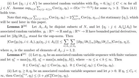
Lemma 2[21](i) Let {ηj: j ∈N} be associated random variables with Eηj=0, supj∈NE|ηj|r0+δ<∞for some r0>2 and δ >0.AssumeO(n?(r0?2)(r0+δ)/(2δ)).Let {aj,j ≥1} be a real constant sequence, a:=supj|aj|<∞.Then

Lemma 5Suppose that Assumptions A1-A5 are satisfied.Then

(4.2) follows if we can verify

By Conditions A1, A2(ii), A3(i)-(ii) and A4,

where we have used

for the identical matrix Ir, which proves (4.5).

where we have used(4.7)and the conditions A2,A3(iii),A4(i)and A5(i).(4.6)is thus verified.

Next we will prove (4.4).To this end, we only need to show, for any given l ∈Rrwith||l||=1, that

We first show that

It follows that

By the proof of Lemma 3.1 in [2] and (4.7), we have

(4.14)-(4.15) imply that

Similarly,

which implies

Again, by the proof of Lemma 3.1 in [2] and (4.7),

Similar to the proof of Theorem 2.1 in [2],

So by Lemma 3, stationarity and (4.7), we have

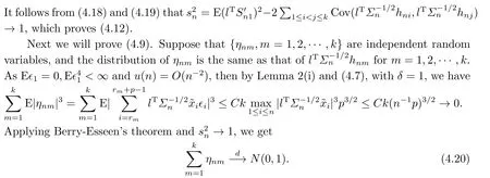
Then (4.9) is implied by (4.20) and (4.21).(4.4) is then verified.

From (4.4)-(4.6) and the Cramer-Wold theorem, we obtain Lemma 5.

Lemma 6Suppose that Assumptions A1-A5 are satisfied.Then

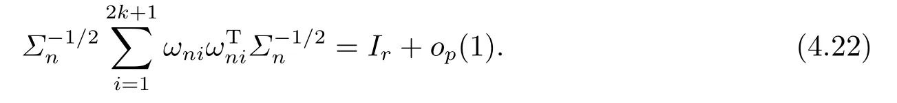
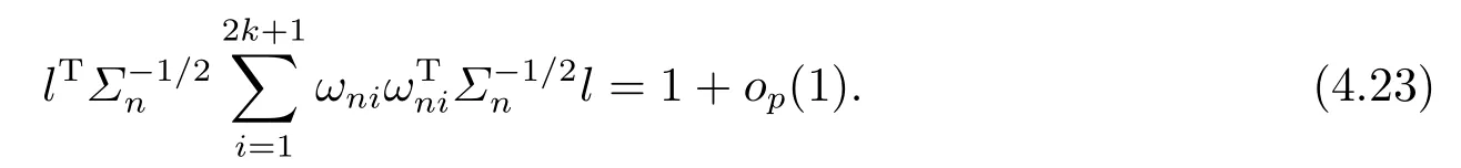
ProofTo prove (4.22), we only need to show that for any l ∈Rrwith ||l||=1,

Note that

then (4.23) follows.

To prove (4.25), it is enough to show that

where

with {hni} being defined in the proof of Lemma 5.Then

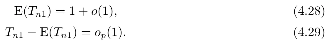
To show (4.28), we only need to prove the following equations.

Obviously, by (4.12), we have

Similar to the proof of (4.13), from (4.7) and the conditions A2 and A4, we have

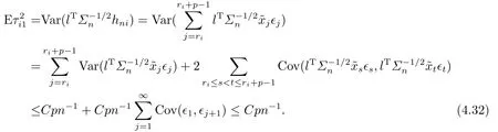
Reviewing the control of the order ofin the proof of Lemma 5, under the conditions A1,A2(ii), A3(i)-(ii), A4 and (4.7),

Similar to the proof of (4.32), by the conditions A2, A3(iii) and A4, we have

In order to prove (4.29), we only need to show the following equations.

It is clear that

By the Markov inequality and the proof of (4.33), we have

Similarly, one can show that

Next, we will show that

To prove (4.42), we will show that

Then

It is clear that{vi1,i ≥1},{vi2,i ≥1}and{vi1+vi2,i ≥1}are all associated random variable sequences.By Lemmas 3 and 4, we have

On the other hand, note thatand by Lemma 4,

Then from Lemma 2(ii), we have

Combining (4.45) and (4.46), we have

Similarly,

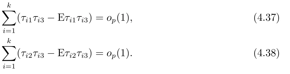
By (4.44)(4.47)-(4.49), we obtain (4.43).Thus (4.39) is proved.From (4.34)-(4.39), we have(4.29).

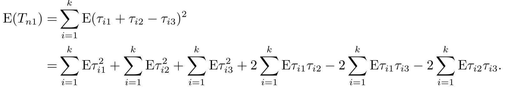
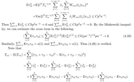
Similar to the proof of (4.25), decomposing ETn2into six terms, then we can prove each term is of order o(1).Therefore, it can been show that ETn2= o(1).Then (4.26) holds true since Tn2is nonnegative.The proof of (4.27) is much less involved than the proof of (4.26) as the size of Tn3is much smaller than that of Tn2.We thus also omit the proof of (4.27).

The proof of Lemma 6 is thus completed.

Proof of Theorem 1Let

We first show the following results

From q ≤Cp,n ?k(p+q)≤Cp, conditions A1, A2(i), A3(i)-(ii) and Lemma 1, we have

We thus have (4.51).

From Lemmas 5 and 6, we have (4.53) and (4.52), respectively.

Using (4.51) to (4.53), similar to the proof of Theorem 1 in [13], one can show that Theorem 1 in this article holds true.