QIAO Mei-hong,LIU An-ping

(1.School of Mathematics&Physics,China University of Geoscience,Wuhan 430074,China)

(2.Center for Mathematical Sciences,Huazhong University of Science and Technology, Wuhan 430074,China)

BIFURCATION IN A RATIO-DEPENDENT PREDATOR-PREY SYSTEM WITH STAGE-STRUCTURED IN THE PREY POPULATION

QIAO Mei-hong1,2,LIU An-ping1

(1.School of Mathematics&Physics,China University of Geoscience,Wuhan 430074,China)

(2.Center for Mathematical Sciences,Huazhong University of Science and Technology, Wuhan 430074,China)

In this paper,we study the bifurcation of ratio-dependent predator-prey system. By using the characteristic equation of the linearized system and the center manifold theorem,we derive the stability of the system and direction of the Hopf bifurcation.

time delay;predator-prey model;stability;Hopf bifurcation

1 Introduction

Over the years,predator-prey models described by the ordinary di ff erential equations (ODEs),which were proposed and studied widely due to the pioneering theoretical works by Lotka[1]and Volterra[2].

A most crucial element in these models is the functional response,the function that describes the number of prey consumed per predator per unit time for given quantities of prey x and predator y.

Arditi and Ginzburg[3]suggested that the essential properties of predator-dependence could be rendered by a simpler form which was called ratio-dependence.The trophic function is assumed to depend on the single variablerather than on the two separate variables x and y.Generally,a ratio-dependent predator-prey model of Arditi and Ginzburg[3]is

In this paper,we will focus our attention on the ratio-dependent type predator-prey

model with Michaelis-Menten type functional response,which takes the form of

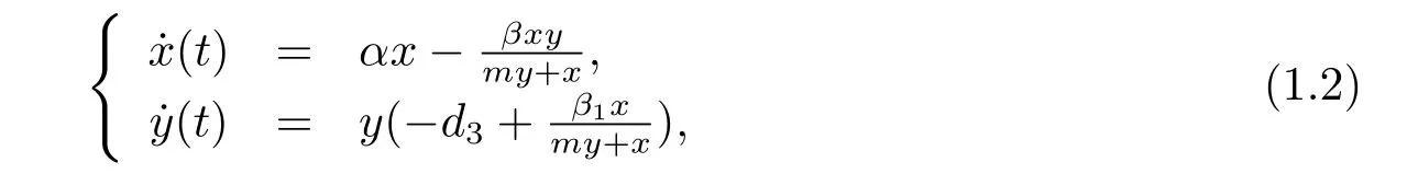
where α,β,m,d3and β1are positive constants;d3,β,m and β1stand for the predator death rate,capturing rate,half saturation constant and conversion rate,respectively.The dynamics of predator-prey system was studied extensively[4-11].

In order to ref l ect that the dynamical behaviors of models that depend on the past history of the system,it is often necessary to incorporate time-delays into the models.Suppose that in a certain environment there are the prey and predator species with respective population densities x(t)and y(t)at time t.

Based on the above discussion,by incorporating age-structure of prey and time delay into system(1.2)and supposing that the predator species captures only the adult prey species,we establish the following model

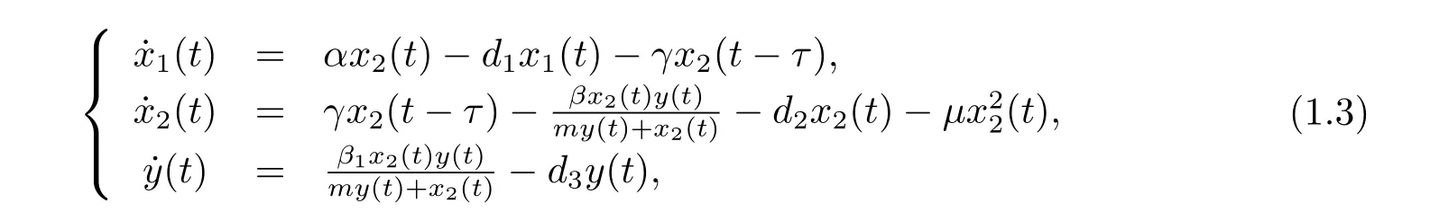
where x1(t),x2(t),y(t)represents the densities of immature prey,mature prey and predator, respectively,α,d1,d2,d3,β,γ,m,μand β1stand for the birth rate of prey,the immature prey death rate,the mature prey death rate,the predator death rate,capturing rate,the conversion rate of immature prey to mature prey,half saturation constant,the density dependence rate of the mature prey and conversion rate,respectively.τ is called the maturation time of the prey species.

2 Stability of a Positive Equilibrium and the Existence of Hopf Bifurcations

In this section,we will discuss the local stability of a positive equilibrium and the existence of Hopf bifurcations in system(1.3).It is easy to deduce that system(1.3)has a unique positive equilibriumif the following holds.

Then we can get the linear part of system(1.3),

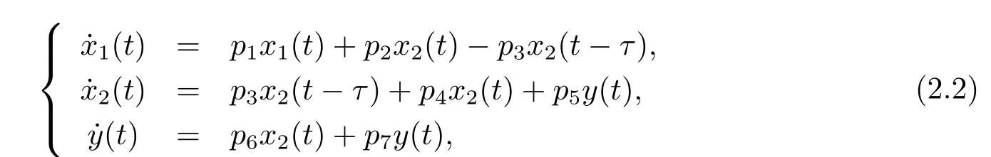
where pi(i=1,2,3,4,5,6,7)are def i ned in(2.1).

Therefore the corresponding characteristic equation[18]of system(2.2)is

It is well-known that the zero steady state of system(2.2)is asymptotically stable if all roots of eq.(2.3)have negative real parts,and is unstable if eq.(2.3)has a root with positive real part.In the following,we will study the distribution of roots of eq.(2.3).

Obviously,λ=p1=-d1＜0 is a negative root of eq.(2.3).

If iω(ω＞0)is a root of eq.(2.3),then

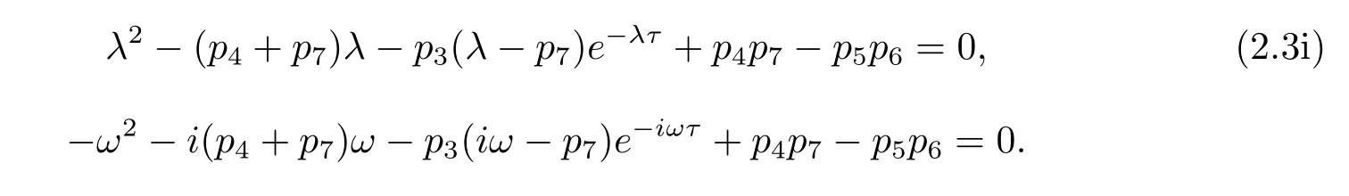
Separating the real and imaginary parts of above formula gives the following equations

which implies that

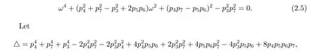
further note that if

Solving for τ0,we get

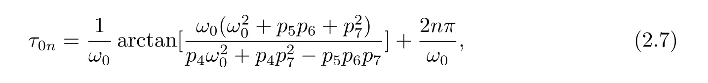
where n=0,1,2,3,···.

The smallest τ0is obtained by choosing n=0,then from(2.5),we get

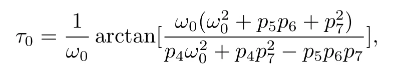
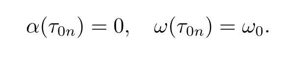
then(τ0n,ω0)solves eq.(2.4).This means that when τ=τ0n,eq.(2.3)has a pair of purely imaginary roots±iω0.

Now let us consider the behavior of roots of eq.(2.3)near τ0n.Denote λ(τ)=α(τ)+ iω(τ)as the root of eq.(2.3)such that

Substituting λ(τ)into eq.(2.3i)and dif f erentiating both sides of it with respect to τ, we have

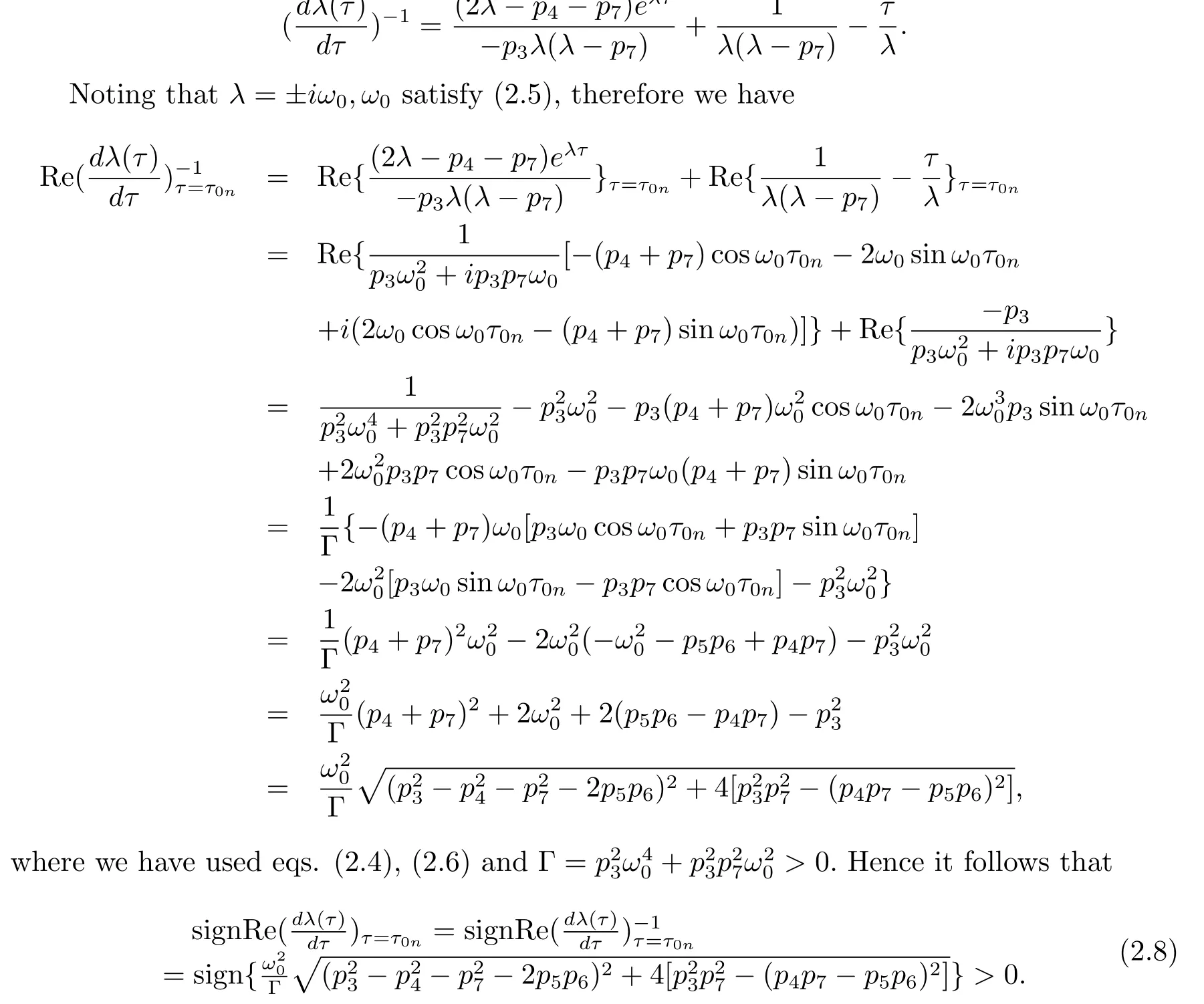
Therefore,when the delay τ near τ0nis increased,the root of eq.(2.3)crosses the imaginary axis from left to right.In addition,note that when τ=0,eq.(2.3)has roots with negative real parts only if

(H3)p3+p4+p7＜0 and p3p7+p4p7-p5p6＞0.

Thus summarizing the above remarks and the well-known Rouche theorem,we have the following results on the distribution of roots of eq.(2.3).

Lemma 2.1 Let τ0n(n=0,1,2,···)be def i ned as in(2.7),then all roots of eq.(2.3) have negative real parts for all τ∈[0,τ0).However,eq.(2.3)has at least one root with positive real part when τ＞τ0,and eq.(2.3)has a pair of purely imaginary root±iω0, when τ=τ0.More detail,for τ∈(τ0n,τ0n+1](n=0,1,2,···),eq.(2.3)has 2(n+1)roots with positive real parts.Moreover,all roots of eq.(2.3)with τ=τ0n(n=0,1,2,···)have negative real parts except±iω0.

Applying Lemma 2.1,Theorem 11.1 developed in[12],we have the following results. Theorem 2.1 Let(H1),(H2)and(H3)hold.Let ω0and τ0n(n=0,1,2,···)be def i ned as in(2.6)and(2.7),respectively.

(i)The positive equilibrium E?of system(1.2)is asymptotically stable for all τ∈[0,τ0) and unstable for τ＞τ0.

(ii)System(1.3)undergoes a Hopf Bifurcation at the positive equilibrium E?when τ=τ0n(n=0,1,2,···).

3 Direction of Hopf Bifurcation

In Section 2,we have proven that system(1.3)has a series of periodic solutions bifurcating from the positive equilibrium E?at the critical values of τ.In this section,we derive explicit formulae to determine the properties of the Hopf bifurcation at critical values τ0nby using the normal form theory and center manifold reduction[13].

Without loss of generality,denote the critical values τ0nbyˉτ,and set τ=ˉτ+μ.Then μ=0 is a Hopf bifurcation value of system(1.3).Thus we can work in the phase space C=C([-ˉτ,0],R3).

Let u1(t)=x1(t)-x?1,u2(t)=x2(t)-x?2,u3(t)=y(t)-y?.Then system(1.3)is transformed into

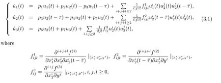
here f(1),f(2)and f(3)are def i ned in(2.1).

For the simplicity of notations,we rewrite(3.1)as

where u(t)=(u1(t),u2(t),u3(t))T∈R3,ut(θ)∈C is def i ned by ut(θ)=u(t+θ),and Lμ：C→R,f：R×C∈R are given by

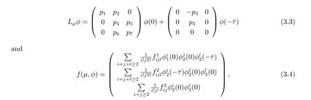
respectively.By Riesz representation theorem,there exists a function η(θ,μ)of bounded variation for θ∈[-ˉτ,0]such that

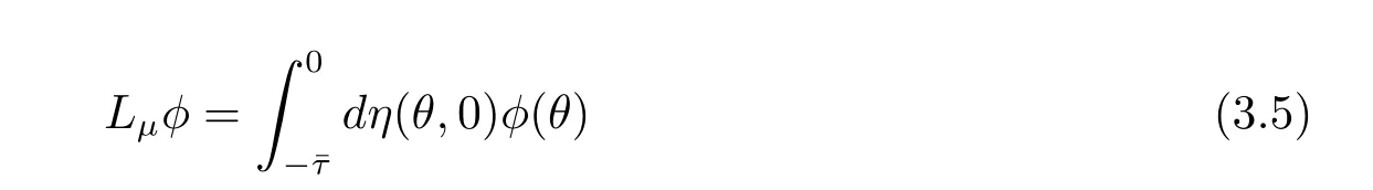
for φ∈C.

In fact,we can choose

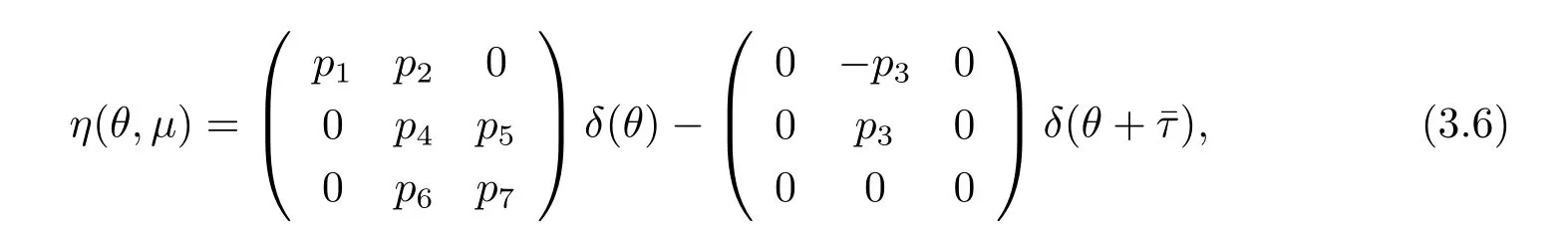
where δ is the vector,whose components are the Dirac delta functions.For φ∈C1([-ˉτ,0],R3), def i ne

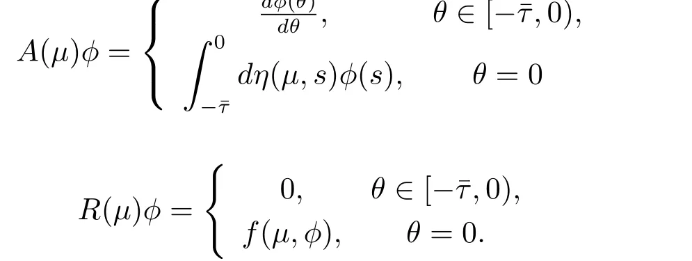
and

Then system(3.2)is equivalent to

where xt(θ)=x(t+θ)for θ∈[-ˉτ,0].

For ψ∈C1([0,ˉτ],(R3)?),def i ne

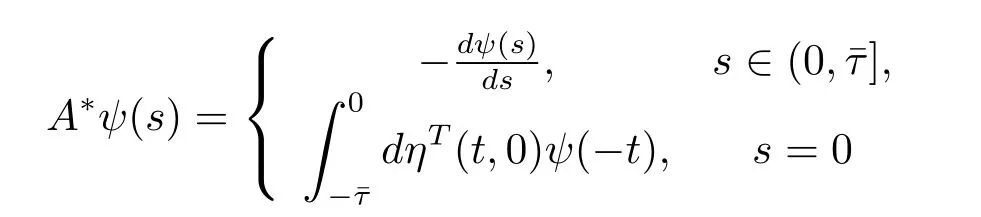
and a bilinear inner product

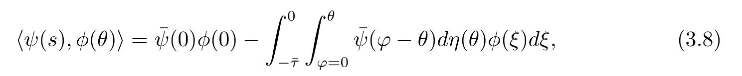
where η(θ)=η(θ,0).Then A(0)and A?are adjoint operators.By discussions in Section 2 and foregoing assumption,we know that±iω0are eigenvalues of A(0).Thus,they are also eigenvalues of A?.We f i rst need to compute the eigenvector of A(0)and A?corresponding to iω0and-iω0,respectively.

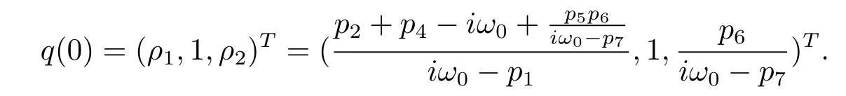
Suppose that q(θ)=(ρ1,1,ρ2)Teiω0θis the eigenvector of A(0),(3.5)and(3.6)that

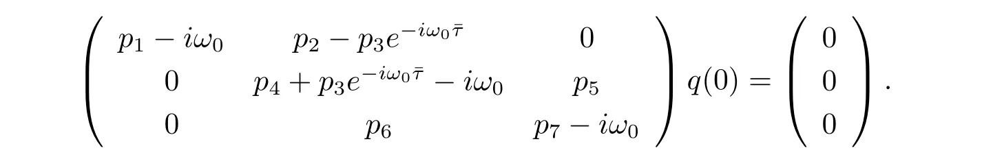
We therefore derive that

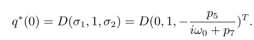
On the other hand,suppose that q?(s)=D(σ1,1,σ2)eiω0sis the eigenvector of A?corresponding to-iω0.From the def i nition of A?,(3.5)and(3.6),we have

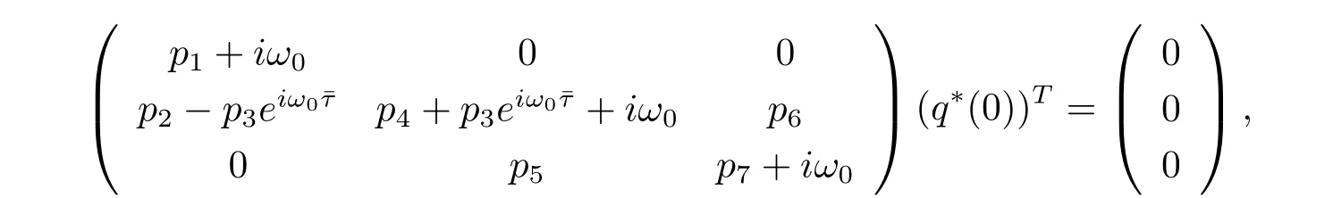
which yields

In order to assure hq?(s),q(θ)i=1,we need to determine the value of D.From(3.7), we have

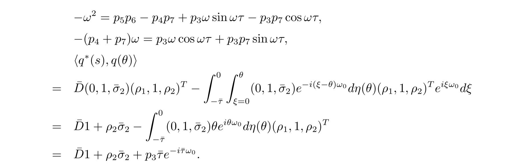
Thus we can choose

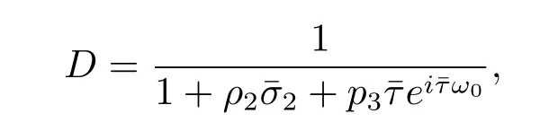
such that hq?(s),q(θ)i=1,hq?(s),ˉq(θ)i=0.

In the remainder of this section,we will compute the coordinates to describe the center manifold C0atμ=0.Let utbe the solution of eq.(3.2)withμ=0.

Def i ne

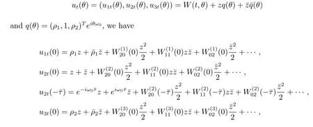
On the center manifold C0,we have W(t,θ)=W(z(t),ˉz(t),θ),where

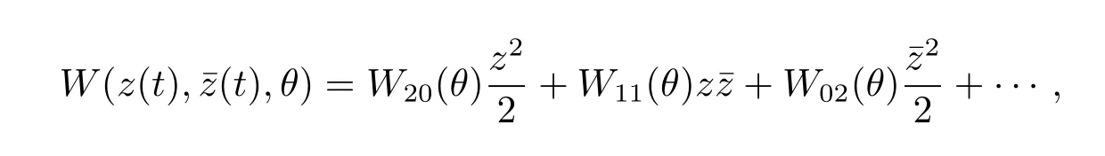
z andˉz are local coordinates for center manifold C0in the direction of q?andˉq?.

Note that W is real if utis real.We only consider real solutions.For the solution ut∈C0of(3.2),sinceμ=0,we have

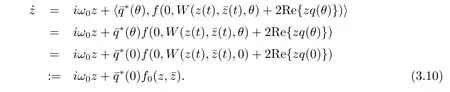
We rewrite(3.10)as˙z=iω0z+g(z,ˉz)with

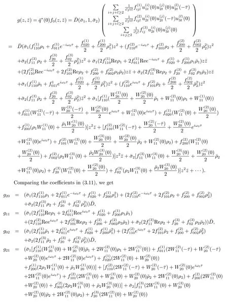
Noting that

thus it follows from(3.4)and(3.11)that

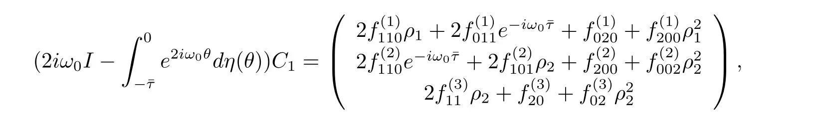
We now compute W20(θ)and W11(θ).It follows from(3.7)and(3.9)that

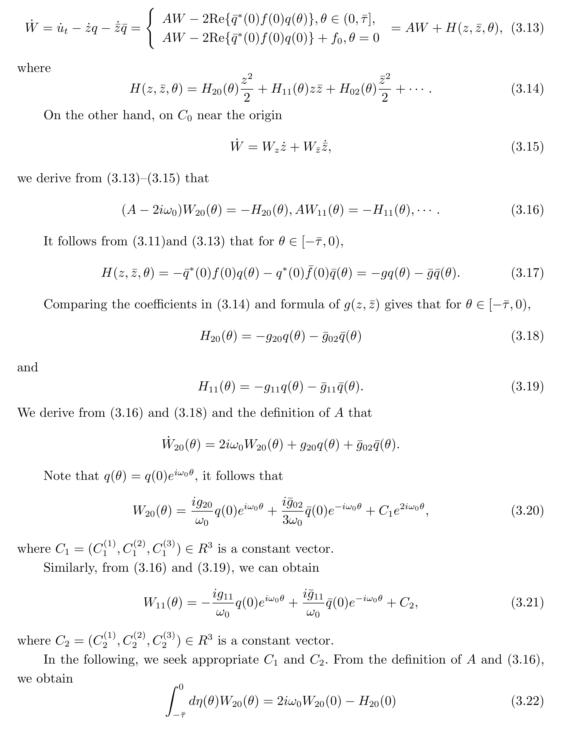
and

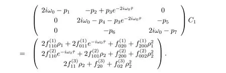
where η(θ)=η(0,θ).From(3.13),it follows that

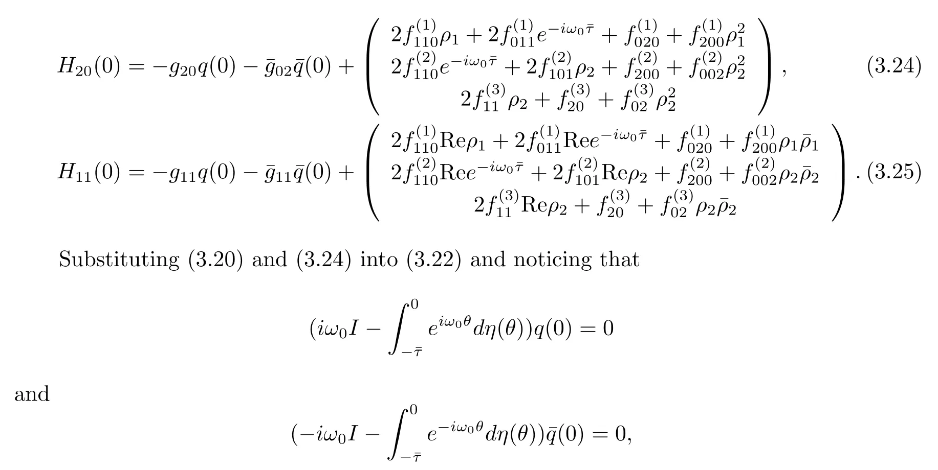
we obtain

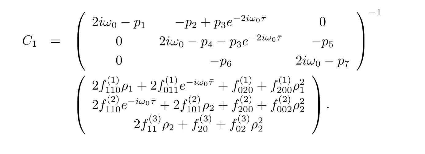
which leads to

It follows that

Similarly,substituting(3.21)and(3.25)into(3.23),we get

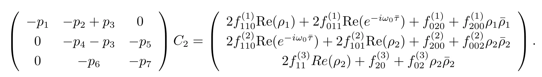
Thus we can determine W20(θ)and W11(θ)from(3.20)and(3.21).Furthermore,we can determine g21.Therefore,each gijin(3.12)is determined by the parameters and delay in system(3.1).Thus we can compute the following values

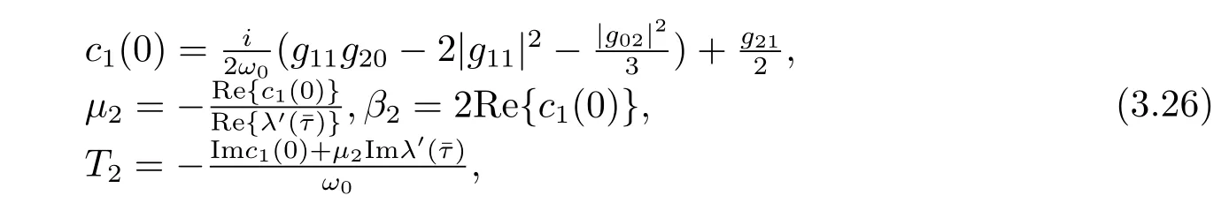
which determine the quantities of bifurcating periodic solutions in the center manifold at the critical valueˉτ,i.e.,μ2determines the direction of the Hopf bifurcation：ifμ2＞0(μ2＜0), then the Hopf bifurcation is supercritical(subcritical)and the bifurcating periodic solutions exist for τ＞ˉτ(τ＜ˉτ);β2determines the stability of the bifurcating periodic solutions：the period increase(decrease)if T2＞0(T2＜0).

From what has been discussed above,we could determine the stability and direction of periodic solutions bifurcating from the positive equilibrium E?at the critical pint τ0n.

[1]Lotka A J.Elements of physical biology[M].New York,Baltimore：Will.Wil.,1925.

[2]Volterra V.Variazionie f l uttuazioni del numero d’individui in specie animali conviventi[J].Mem. Acad.Licei.,1926,2：31-113.

[3]Arditi R,Ginzburg L R.Coupling in predator-prey dynamics：ratio-dependence[J].J.Theor.Biol., 1989,139：311-326.

[4]Berezovskaya F,Karev G,Arditi R.Parametric analysis of the ratio-dependent predator-prey model[J].J.Math.Biol.,2001,43：221-246.

[5]Hsu S B,Hwang T W,Kuang Y.Global analysis of the Michaelis-Menten type ratio dependent predator-prey system[J].J.Math.Biol.,2001,42：489-506.

[6]Jost C,Arino O,Arditi R.About deterministic extinction in ratio-dependent predator-prey models[J].Bull.Math.Biol.,1999,61：19-32.

[7]Ruan S,Wolkowicz G S K,Wu J.Dif f erential equations with applications to biology[J].Fields Inst. Commun.,Providence,RI：AMS,1999,21：325-337.

[8]Kuang Y,Beretta E.Global qualitative analysis of a ratio-dependent predator-prey system[J].J. Math.Biol.,1998,36：389-406.

[9]Gao S J,Chen L S,Teng Z D.Hopf bifurcation and global stability for a delayed predator-prey system with stage structure for predator[J].Appl.Math.Comput.,2008,202：721-729.

[10]Qiao M H,Liu A P.Qualitative analysis for a Reaction-dif f usion predator-prey model with disease in the prey species[J].J.Appl.Math.,Article ID：236208,2014.

[11]Urszula F,Qiao M H,Liu A P.Asymptotic dynamics of a deterministic and stochastic predator-prey model with disease in the prey species[J].Math.Meth.Appl.Sci.,2014,37(3)：306-320.

[12]Zhang F Q,Zhang Y J.Hopf bifurcation for Lotka-Volterra Mutualist systems with three time delays[J].J.Biomath.,2011,26(2)：223-233.

[13]Hale J,Lunel S.Introduction to functional dif f erential equations[M].New York：Springer-Verlag, 1993.

[14]Hassard B,Kazarinof fD,Wan Y.Theory and applications of Hopf bifurcation[M].Cambridge：Cambridge University Press,1981.

[15]Zhou L,Shawgy H.Stability and Hopf Bifurcation for a competition delay model with dif f usion[J]. J.Math.,1999,19(4)：441-446.

[16]Keeling M J,Grenfell B T.Ef f ect of variability in infection period on the persistence and spatial spread of infectious diseases[J].Math.Biosci.,1998,147(2)：207-226.

[17]Natali H.Stability analysis of Volterra integral equations with applications to age-structured population models[J].Nonl.Anal.,2009,71：2298-2304.

[18]David A.Sanchez,ODEs and stability theory[M].Mineola,New York：Dover Publ.,2012.

具有比率依賴和年齡結(jié)構(gòu)的捕食食餌系統(tǒng)的分支研究

喬梅紅1,2,劉安平1

(1.中國(guó)地質(zhì)大學(xué)(武漢)數(shù)理學(xué)院,湖北武漢430074)
(2.華中科技大學(xué)數(shù)學(xué)中心,湖北武漢430074)

本文研究了具有比率依賴的捕食食餌的分支問(wèn)題.利用線性特征方程的方法,獲得了方程解的穩(wěn)定性結(jié)果,得到了Hopf分支的方向和穩(wěn)定性的充分條件.

時(shí)滯;捕食食餌模型;穩(wěn)定性;Hopf分支

O175.13

A

0255-7797(2017)05-0956-13

?Received date：2014-07-26Accepted date：2015-01-04

Supported by the Basic Research Program of Hubei Province(2014CFB898); NSFC(11571326;11601496).

Biography：Qiao Hongmei(1982-),female,born at Linfen,Shanxi,lecturer,major in biomathematics.

2010 MR Subject Classif i cation：34D20