
Two Generalized Successive Overrelaxation Methods for Solving Absolute Value Equations
2020-07-08 03:25:16RashidAliPanKejiaAsadAli
數(shù)學(xué)理論與應(yīng)用 2020年4期
Rashid Ali Pan Kejia Asad Ali
(1.School of Mathematics and Statistics, Central South University, Changsha 410083, China;2.Department of Mathematics, Abdul Wali Khan University Mardan 23200, KPK Pakistan)
Abstract Many problems in operations research, management science, and engineering fields lead to solve absolute value equations.In this paper, we suggest and analyze two new methods called generalized successive overrelaxation(GSOR)method and modified generalized successive overrelaxation(MGSOR)method for solving the absolute value equations Ax-|x|=b, where A∈Rn×n is an arbitrary real matrix.Also, we study the convergence properties of the suggested methods.Lastly, we end our paper with numerical examples that show that the given methods are valid and effective for solving absolute value equations.
Key words Absolute value equation GSOR method MGSOR method Numerical experiment
1 Introduction
Consider the absolute value equation(AVE)with matrixA∈Rn×n,b∈Rnand |*| indicates the absolute value given by
Ax-|x|=b.
(1)
The AVEs are one of the important nonlinear and non-differentiable systems which arise in optimization, such as the bimatrix games, the linear and quadratic programming, the contact problems, the network prices, the network equilibrium problems; see[1-6,11,12,16,26,29,34]and the references therein.Therefore, the study of efficient numerical algorithms and theories for AVEs is of great importance.
The AVE is also equivalently reformulated to linear complementarity problem(LCP)and mixed integer programming; see[14,18,19,21,22,25,32]and the references therein.For example, consider the LCP(M,q)of finding a vectorz∈Rn, such that
z≥0, Φ=(Mz+q)≥0,zTΦ=0,
(2)
whereM∈Rn×nandq∈Rn.The above LCP(2)can be demoted to the following AVE
Ax-B|x|=q,
(3)
with
whereA=(M+I)andB=(M-I).Mezzadri[20]presented the equivalence between AVEs and horizontal LCPs.Prokopyev[28]has presented the unique solvability of AVE, and its connections with mixed integer programming and LCP.Mangasarian[23]has determined that AVE is equivalent to a concave minimization problem and examined the latter problem instead of AVE.Hu and Huang[15]reformulated the AVE system to the standard LCP and provided some outcomes for the solution of AVE(1).
xi+1=A-1(|xi|+b),i=0,1,2,…,
wherex0=A-1bis the initial vector.Ke and Ma[17]suggested an SOR-like method to solve the AVE(1).This method can be summarized as follows:
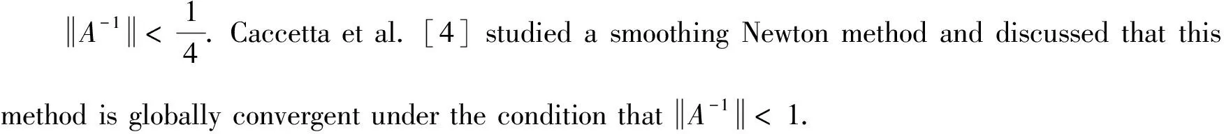
Dong et al.[7]further studied the SOR-like method for solving(1)and presented some novel convergence properties which are different from the results of[17].Nguyen et al.[27]presented unified smoothing functions associated with second-order cone for solving(1).Hashemi and Ketabchi[13]proposed the numerical comparisons of smoothing functions for the system of AVEs.
The paper is prepared as follows.In Sec.2, various notations and definitions are presented that would be used throughout this paper.In Sec.3, we present the proposed methods and their convergence for solving AVE(1).Numerical results and concluding remarks are given in Secs.4 and 5, respectively.
2 Preparatory Knowledge
Here, we briefly review some notations and concepts used in this paper.
LetA=(aij)∈Rn×nandC=(cij)∈Rn×n, we writeA≥0 ifaij≥0 holds for all 1≤i,j≤nandA≥CifA-C≥0.We express the absolute value and norm ofA∈Rn×nas |A|=(|aij|)and ‖A‖∞, respectively.The matrixA∈Rn×nis called anZ-matrix ifaij≤0 fori≠j, and anM-matrix if it is a nonsingularZ-matrix and withA-1≥0.
3 Proposed Methods
In this section, we discuss the proposed methods.This section contains two parts, the first part includes the GSOR method and its convergence, and the second part includes the MGSOR method and its convergence for solving AVEs.
3.1 GSOR method for AVE
Recalling that the AVE(1)has the following form
Ax-|x|=b.
Multiplyingλ, we get
λAx-λ|x|=λb.
(4)
Let
A=DA-LA-UA,
(5)
where,DA,LAandUAare diagonal, strictly lower and upper triangular parts of A, respectively.Using(4)and(5), the GSOR method is suggested as:
(DA-λLA)x-λ|x|=((1-λ)DA+λUA)x+λb.
(6)
Using the iterative scheme,(6)can be written as
(DA-λLA)xi+1-λ|xi+1|=((1-λ)DA+λUA)xi+λb,
(7)
wherei=0,1,2,…, and 0<λ<2.
For choices ofλwithλ∈(0,1), these methods are called underrelaxation methods; forλ=1,(7)is reduced to the GGS method[8].In this paper, we are interested in choosingλwithλ∈(1,2), these are called overrelaxation methods.
Algorithm 3.1
Step 1: Select a parameterλ, initial vectorx0∈Rnand seti=0.
Step 2: Calculate
yi=A-1(|xi|+b),
Step 3: Calculate
xi+1=λ(DA-λLA)-1|yi|+(D-λLA)-1[((1-λ)DA+λUA)xi+λb].
Step 4: Ifxi+1=xi, then stop.If not, seti=i+1 and return to step 2.
Now, the following theorem indicates the convergence of the GSOR method.
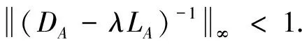
Theorem 3.1Suppose that(1)is solvable.Let the diagonal values ofA>1 andDA-LA-Imatrix is the strictly row wise diagonally dominant.If
(8)
then the sequence {xi} of GSOR method converges to the unique solutionx*of AVE(1).
0≤|λLA|t<(DA-I)t,
if we take
|λLA|t<(DA-I)t.
(9)
0≤|(I-Q)-1|=|I+Q+Q2+Q3+…+Qn-1|
≤(I+|Q|+|Q|2+|Q|3+…+|Q|n-1)=(I-|Q|)-1.
(10)
Thus, from(9)and(10), we get
<(I-|Q|)-1(I-|Q|)t=t.
So, we obtain
For the uniqueness of the solution, letx*andz*be two distinct solutions of the AVE(1).Using(6), we get
x*=λ(DA-λLA)-1|x*|+(DA-λLA)-1[((1-λ)DA+λUA)x*+λb],
(11)
z*=λ(DA-λLA)-1|z*|+(DA-λLA)-1[((1-λ)DA+λUA)z*+λb].
(12)
From(11)and(12), we get
x*-z*=λ(DA-λLA)-1(|x*|-|z*|)+(DA-λLA)-1((1-λ)DA+λUA)(x*-z*).
Using Lemma 2.1 and(8), the above equation can be written as
which leads to a contradiction.Hence,x*=z*.
For convergence, letx*is a unique solution of AVE(1).Consequently, from(11)and
xi+1=λ(DA-λLA)-1|xi+1|+(D-λLA)-1[((1-λ)DA+λUA)xi+λb],
we deduce
xi+1-x*=λ(DA-λLA)-1(|xi+1|-x*)+(DA-λLA)-1[((1-λ)DA+λUA)(xi-x*)].
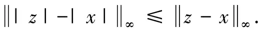
Taking infinity norm and using Lemma 2.1, we obtain
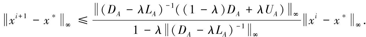
This inequality indicates that the convergence of the method is obtained if condition(8)is satisfied.
3.2 MGSOR method for AVE
In this unit, we present the MGSOR method.By using(4)and(5), we can define the MGSOR iteration method for solving(1)as follows:
(DA-λLA)xi+1-λ|xi+1|=((1-λ)DA+λUA)xi+1+λb,i=0,1,2,….
Algorithm 3.2
Step 1: Select a parameterλ, initial vectorx0∈Rnand seti=0.
Step 2: CalculateTi=A-1(|xi|+b).
Step 3: Calculate
xi+1=λ(DA-λLA)-1|Ti|+(DA-λLA)-1[((1-λ)DA+λUA)Ti+λb].
Step 4: Ifxi+1=xi, then stop.If not, seti=i+1 and go to step 2.
Now, the following theorem indicates the convergence of the MGSOR method.
Theorem 3.2Suppose that(1)is solvable.IfA>1 andDA-LA-Iis row diagonally dominant, then the sequence of MGSOR method converges to the unique solutionx*of AVE(1).
ProofThe uniqueness follows from Theorem 3.1 directly.To prove the convergence, consider
xi+1-x*=λ(DA-λLA)-1|xi+1|+(DA-λLA)-1[((1-λ)DA+λUA)xi+1+λb]
-(λ(DA-λLA)-1|x*|+(DA-λLA)-1[((1-λ)DA+λUA)x*+λb]),
(DA-λLA)(|xi+1|-|x*|)=λ(xi+1-x*)+((1-λ)DA+λUA)(xi+1-x*),
λ(DA-LA-UA)xi+1-λ|xi+1|=λ(DA-LA-UA)x*-λ|x*|,
(DA-LA-UA)xi+1-|xi+1|=(DA-LA-UA)x*-|x*|.
(13)
From(5)and(13), we have
Axi+1-|xi+1|=Ax*-|x*|,
Axi+1-|xi+1|=b.
Hencexi+1solves system of AVE(1).
4 Numerical experiments
In this unit, we experimentally study the performance of the novel methods of solving the AVEs.All the experiments are presented with Intel(C)Core(TM)i7-7700HQ, CPU @ 2.80 GHz×4, 20 GB RAM, and the codes are written in Matlab(R2017a).Both examples started from the null vector,ω=1,λ=1.1, and the termination condition is given by
Example 4.1Let
andb=Ax*-|x*|∈Rn.The numerical results are given in Table 1.

Table 1 Numerical data of example 4.1
In Table 1, we report the number of iterations(Iter), CPU times in seconds(Time), and residual(RES)of all methods.From the results in Table 1, we notice that the suggested methods can rapidly calculate the AVE solution under some conditions.Also, we taken=1000 and 6000(problem sizes)of example 4.1 and compare all methods graphically.Graphical results are illustrated in Fig.1.
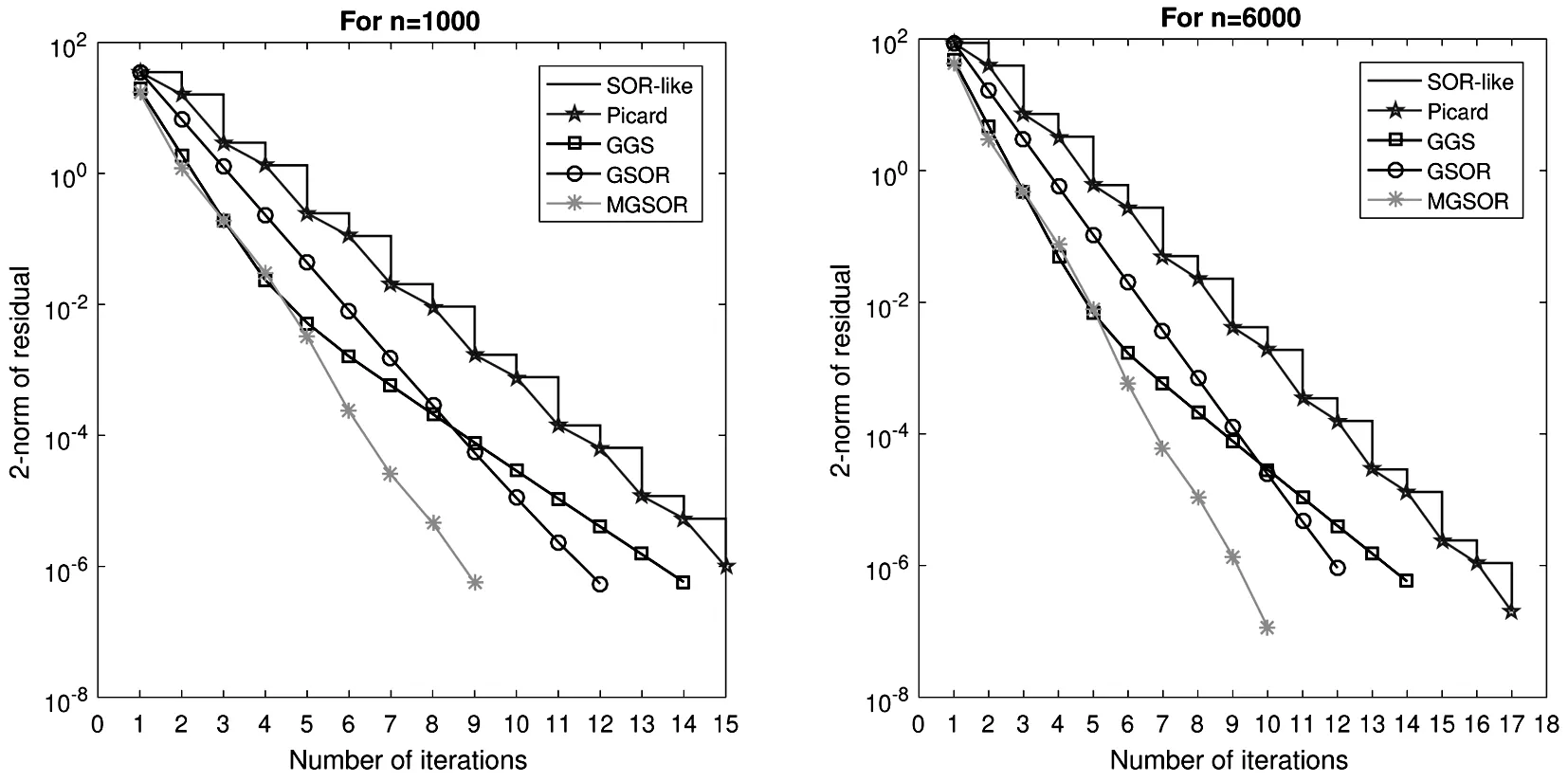
Figure 1 Convergence curves of example 4.1 with different methods
The convergence curves of Fig.1 show the effectiveness of the given methods.Graphical representation illustrates that the convergence of the suggested methods is better than other known methods.
Example 4.2LetA=M+ΨI∈Rn×nandb=Ax*-|x*|∈Rn, such that
whereI∈Rv×vis the identity matrix,n=v2, and
is a tridiagonal matrix.The numerical results are reported in Table 2.In this example, we taken=100 and 900(problem sizes)and compare all methods graphically.Graphical results are presented in Fig.2.

Table 2 Numerical data of example 4.2 with Ψ=4
From Table 2, we see that the “Iter” and “Time” of the proposed methods are less than other known methods.Also, the convergence curves of Fig.2 show the efficiency of the proposed methods.Finally, we conclude that our proposed methods are feasible and effective for AVEs.
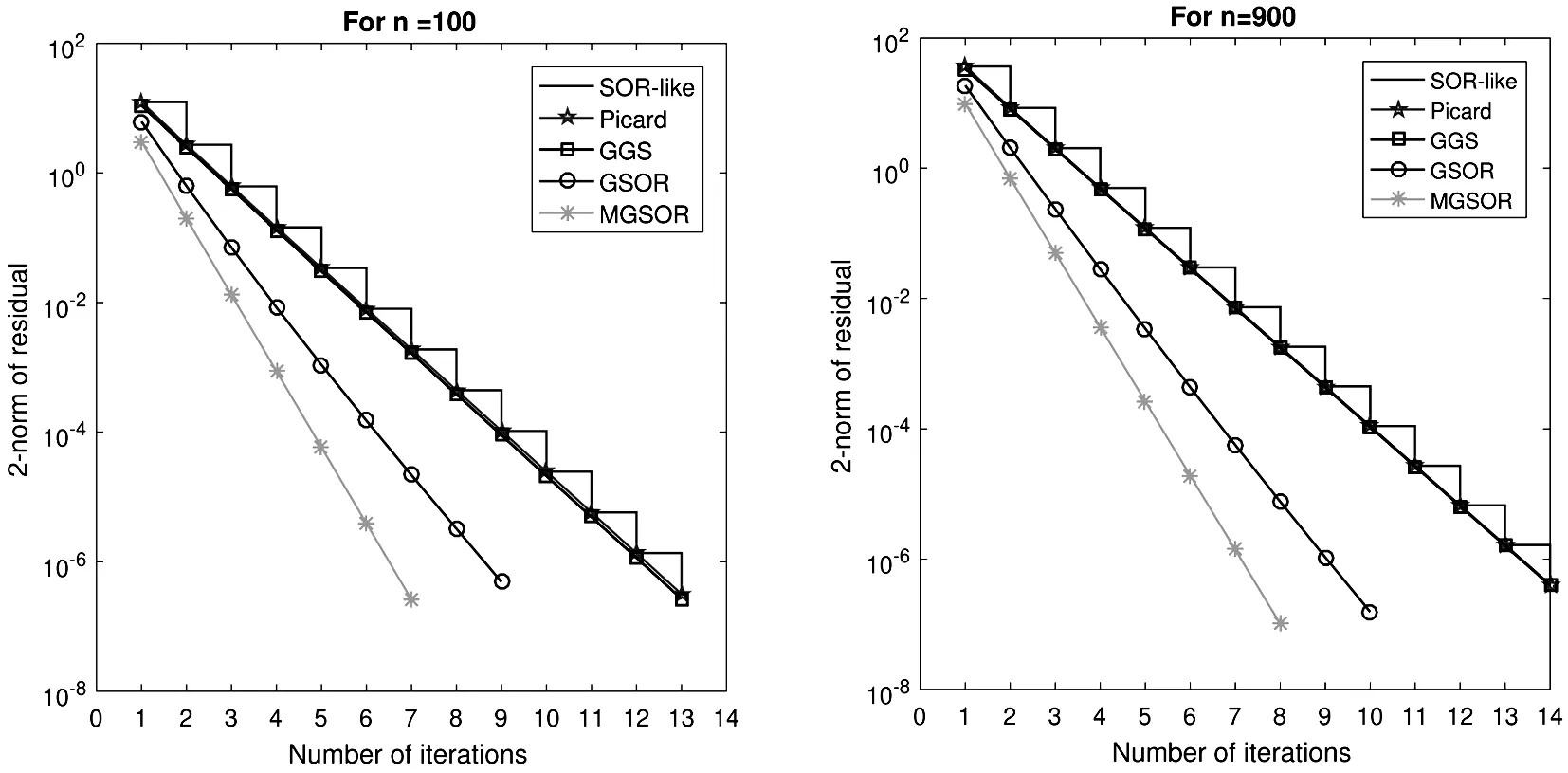
Figure 2 Convergence curves of example 4.2 with different methods
5 Conclusions
In this paper, we studied two new methods which are called the generalized SOR(GSOR)method and the modified generalized SOR(MGSOR)method for solving AVEs, and examined the sufficient conditions for the convergence of the proposed iteration methods.These new iterative methods are very simple and easy to implement.The future work is to extend this idea by taking two more points.Both theoretical analyses and numerical experiments have shown that the suggested algorithms seem promising for solving the AVEs.
 數(shù)學(xué)理論與應(yīng)用2020年4期
- 數(shù)學(xué)理論與應(yīng)用的其它文章
- 基于排隊(duì)論的機(jī)場(chǎng)上客區(qū)系統(tǒng)效益優(yōu)化研究
- The Twin Domination Number of Cartesian Product of Directed Cycle and Path
- An Isolated Toughness Condition for All Fractional(g,f,n,m)-Critical Deleted Graphs
- The Isomorphic Classes of Small Degree Cayley Graphs over Dicyclic Groups
- 非正規(guī)子群彼此同構(gòu)的有限群
- 兩類具有2-等變性的Liénard系統(tǒng)的全局動(dòng)力學(xué)